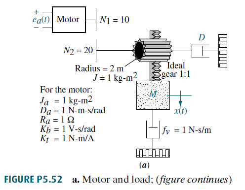
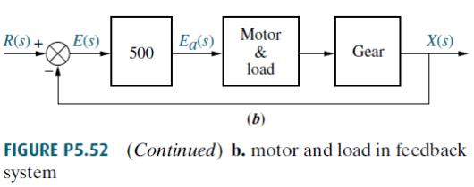
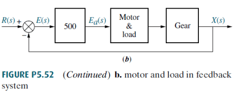
The mechanical system shown in Figure P5.52(a) is used as part of the unity feedback system shown in Figure P5.52(b). Find the values of M and D to yield 20% overshoot and 2 seconds settling time.
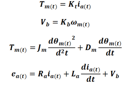
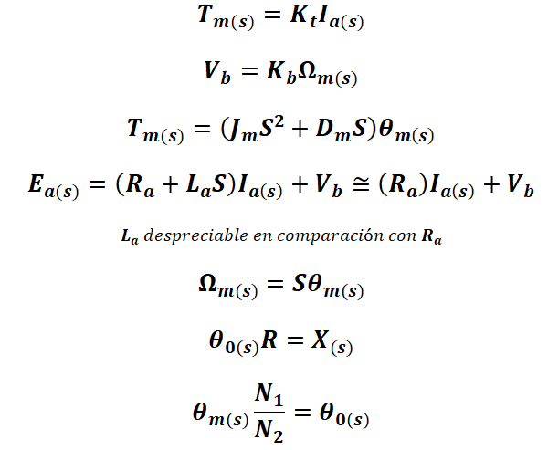
1. System Dynamic
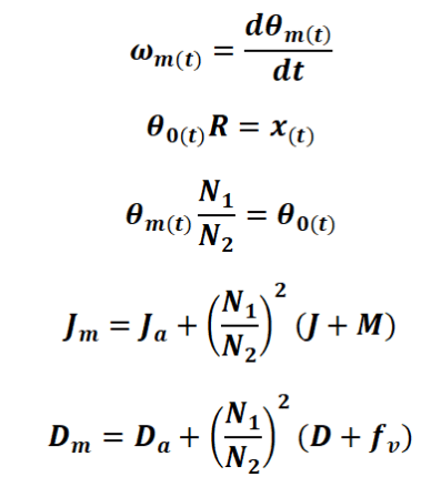
where:
2. Laplace Transform
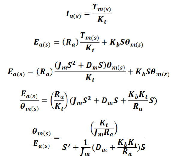
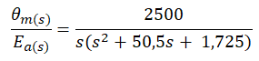
3. Motor&Load Transfer Function (θm(s)/Ea(s))
4. Direct Transfer Function
For the system:
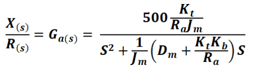
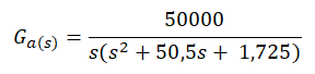
The open-loop transfer function Ga(s) is:
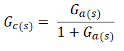
5. Closed-loop transfer function
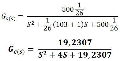
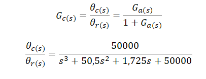
The closed-loop transfer function Gc(s) is:
That is to say:
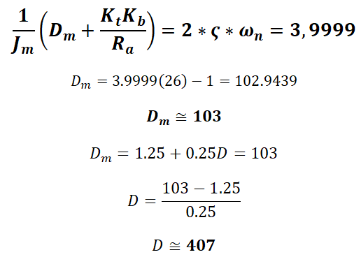
6. Calculation of M and D
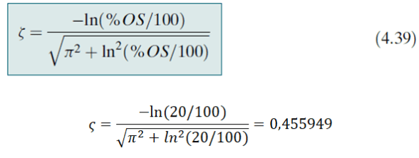
According to:
Besides:
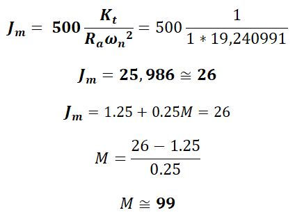
In this way:
Meanwhile:
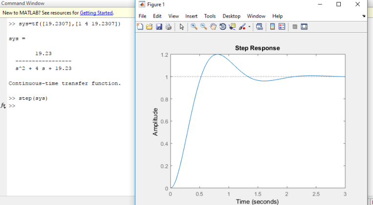
7. Matlab verification
We use Matlab to corroborate replacing all the values calculated in the original transfer function:
Find the values of M and D to yield 20% overshoot and 2 seconds settling time.
>> stepinfo (sys)
RiseTime: 0.3554
SettlingTime: 1.8989
SettlingMin: 0.9331
SettlingMax: 1.1999
Overshoot: 19.9890
Undershoot: 0
Peak: 1.1999
PeakTime: 0.8059
Written by Larry Francis Obando – Technical Specialist – Educational Content Writer
Mentoring Academic / Entrepreneur / Business
Copywriting, Content Marketing, White Papers (Spanish – English)
Escuela de Ingeniería Eléctrica de la Universidad Central de Venezuela, CCs.
Escuela de Ingeniería Electrónica de la Universidad Simón Bolívar, Valle de Sartenejas.
Escuela de Turismo de la Universidad Simón Bolívar, Núcleo Litoral.
Contact: Caracas, Quito, Guayaquil, Jaén, Villafranca de Ordizia- Telf. +34633129287
Find in generic terms, the transfer function of the unit feedback system shown in Figure P5.52 (b) of which the electromechanical system of Figure P5.52 (a) is a part.
1. System Dynamic
where:
2. Laplace Transform
3. Motor&Load Transfer Function (θm(s)/Ea(s))
4. Direct Transfer Function
For the system:
The open-loop transfer function Ga(s) is:
5. Closed-loop transfer function
The closed-loop transfer function Gc(s) is:
That is to say:
This problem is the first part of one where the transient response is requested so that the overshoot is 20% and the settling time is 2 seconds, see the complete problem in the following link: Example 1 – Transient response of an electromechanical system
Written by Larry Francis Obando – Technical Specialist – Educational Content Writer
Mentoring Academic / Entrepreneur / Business
Copywriting, Content Marketing, White Papers (Spanish – English)
Escuela de Ingeniería Eléctrica de la Universidad Central de Venezuela, CCs.
Escuela de Ingeniería Electrónica de la Universidad Simón Bolívar, Valle de Sartenejas.
Escuela de Turismo de la Universidad Simón Bolívar, Núcleo Litoral.
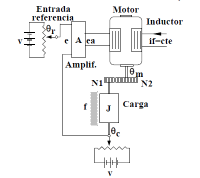
Obtain the mathematical model of the position control system of the figure. Get the block diagram and the ansfer function between the angle of the load and the reference angle θc(s)/θc(s).
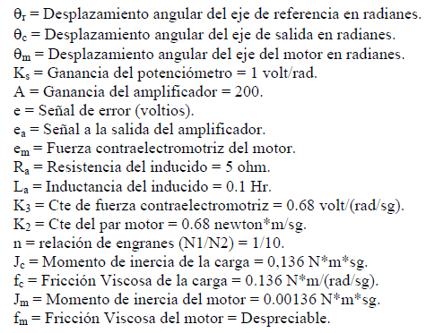
Data:
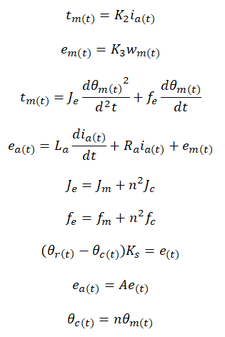
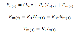
1. System dynamic
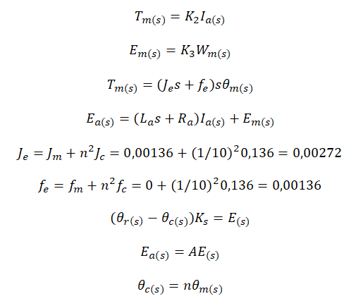
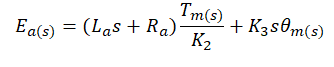
2. Laplace Transform
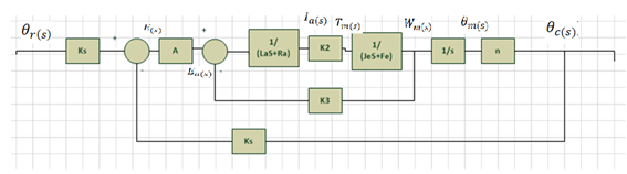
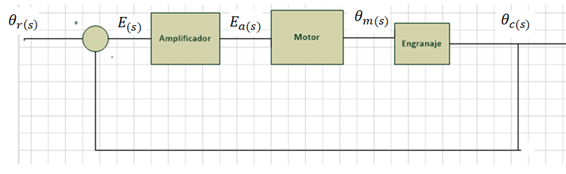
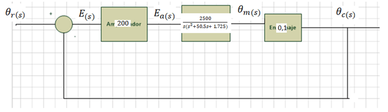
3. Block Diagram
Simplifying conveniently to obtain a model whose transfer function is known:
4. Transfer function of each block of the previous diagram.
Starting from:
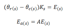
We obtain the following:Then, using:
and substituting, we obtain:
Substituting the value of the data in the previous equation, we obtain:
Simplifying:
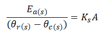
On the other hand, the gain of the amplifier is obtained using:
From where:
Finally, the gear constant is given by the data and is n = 1/10. We then obtain a block diagram with the following transfer functions:
5. System Transfer function.
The open-loop transfer function Ga(s) of the system shown in the previous diagram is:
From where we can easily obtain the closed-loop transfer function Gc (s), which is what the statement asked, using the unit feedback:
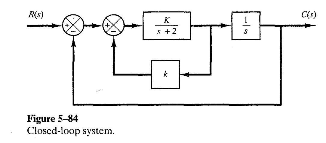
Determinar los valores de K y k tal que el sistema tenga un factor de amortiguamiento relativo ζ de 0.7 y una frecuencia natural ωn de 4 rad/s.
RESPUESTA
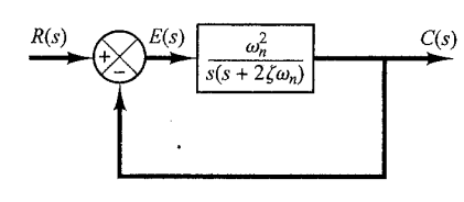
1. Lo primero que se aconseja hacer es obtener el modelo del sistema de la Figura 5-84 que sea equivalente al sistema de segundo orden prototipo, el cual es el siguiente:
Modelo Prototipo
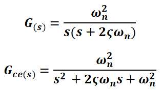
Donde definimos la función de transferencia directa G(s) y la función de transferencia a lazo cerrado Gce(s) como sigue:
2. Determinamos G(s) y Gce(s) en relación al sistema de la Figura 5-84:
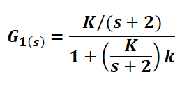
Donde G1(s) es la función de transferencia del lazo cerrado interno formado por K/(s+2) y k:
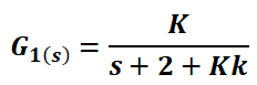
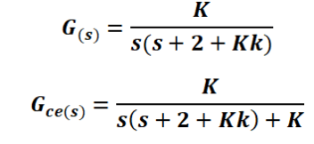
Luego, sustituimos G1(s) en la ecuación de G(s). Actuando de esta manera, obtenemos las funciones de transferencia del sistema de la Figura 5-84, equivalentes al sistema prototipo:
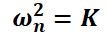
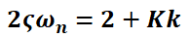
3. Con estas dos funciones podemos obtener lo parámetros que se solicitan en el enunciado, es decir, K y k tal que el sistema tenga un factor de amortiguamiento relativo ζ de 0.7 y una frecuencia natural ωn de 4 rad/s. Para ello comparamos G(s) y Gce(s) obtenidos en el paso 1 con los obtenidos en el paso 2. Así obtenemos que:
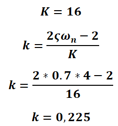
Sustituyendo los valores de las variables aportadas en el enunciado, y despejando, obtenemos el siguiente resultado:
Servicio de Emergencias: Se resuelven ejercicios de Sistemas de Primer y Segundo Orden, con carácter de Urgencia. EN MENOS DE 24 HORAS (precio aprox. por cada ejercicio (o cada pregunta): 13.7 euros) Clases Online: Te Enseño este tema con paciencia y pedagogía. Podemos resolver ejercicios durante la clase (14.7 euros la hora) Contacto: Prof. Larry, Whatsapp: +34613406484, +34633129287 dademuch@gmail.com Otras áreas: Análisis Sistemas, Procesamiento de Señales, Simulación Matlab/Simulink, Sistemas de Control, Modelo y Análisis Matemático de Sistemas Eléctricos, Electrónicos, Mecánicos (MRA), Electromecánicos…
Elaborado por: Larry Francis Obando – Technical Specialist – Educational Content Writer
Mentoring Académico / Emprendedores / Empresarial
Copywriting, Content Marketing, Tesis, Monografías, Paper Académicos, White Papers (Español – Inglés)
Escuela de Ingeniería Eléctrica de la Universidad Central de Venezuela, Caracas.
Escuela de Ingeniería Electrónica de la Universidad Simón Bolívar, Valle de Sartenejas.
Escuela de Turismo de la Universidad Simón Bolívar, Núcleo Litoral.
Si lo que Usted necesita es reducir un Diagrama de Bloques complejo, resolver con urgencia un problema de “Sistema Masa-Resorte-Amortiguador” (encontrar la salida X(t), gráficas en Matlab del sistema de 2do Orden y parámetros relevantes, etc.), o resolver un problema más complejo que involucra el uso de dispositivos electromecánicos (motor, sensor, etc) en un sistema de control…para entregar a su profesor en dos o tres días, o con mayor urgencia…o simplemente necesita un asesor para resolver el problema y estudiar para el próximo examen…envíeme el problema..Yo le resolveré cualquier problema de Sistemas de Control, le entrego la respuesta en digital y le brindo una video-conferencia para explicarle la solución…incluye además simulación en Matlab.
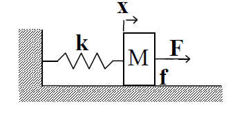
Dada la respuesta del siguiente sistema a una entrada escalón unitario, calcular k, f y M.
RESPUESTA
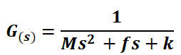
La función de transferencia del sistema es:
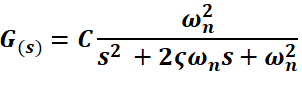
El sistema de segundo orden prototipo tiene la siguiente forma:
Donde C es una constante.
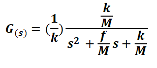
El sistema equivalente queda expresado como:
Donde:
Por tanto:
Por lo que:
Siendo:
Si suponemos que la curva de la gráfica se corresponde con la función y(t), entonces de la gráfica sabemos que el sobrepaso Mp es:
Por otra parte, en términos del factor de amortiguamiento relativo, Mp es:
De donde:
Luego, de la gráfica sabemos que:
Por tanto:
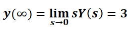
Aplicando el teorema del valor final y observando el comportamiento de y(t) cuando t tiende a infinito:
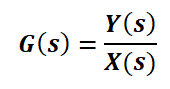
La función de transferencia G(s) nos permite desplegar la expresión para Y(s):
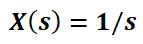
Como la entrada es un escalón unitario:
Por tanto:
Así, volviendo al teorema del valor final:
De donde:
Así:
Es decir:
Regresando a la expresión para la frecuencia natural:
Por último,
Revisión literaria hecha por:
Prof. Larry Francis Obando – Technical Specialist – Educational Content Writer

 That is to say: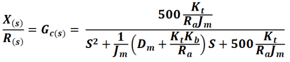
 We obtain the following:
 Then, using: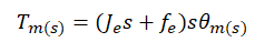





 El sistema de segundo orden prototipo tiene la siguiente forma:
 Donde C es una constante.
El sistema equivalente queda expresado como:
Donde C es una constante.
El sistema equivalente queda expresado como:
 Donde:
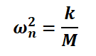 Por tanto:
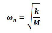 Por lo que:
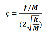
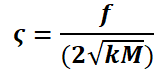 Siendo:
 Si suponemos que la curva de la gráfica se corresponde con la función y(t), entonces de la gráfica sabemos que el sobrepaso Mp es:
 Por otra parte, en términos del factor de amortiguamiento relativo, Mp es:
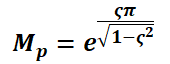
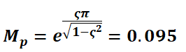 De donde:
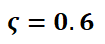 Luego, de la gráfica sabemos que:
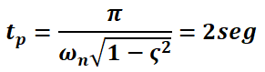 Por tanto:
 Aplicando el teorema del valor final y observando el comportamiento de y(t) cuando t tiende a infinito:
 La función de transferencia G(s) nos permite desplegar la expresión para Y(s):
 Como la entrada es un escalón unitario:
 Por tanto:
 Así, volviendo al teorema del valor final:
 De donde:
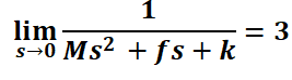 Así:
Así:
 Es decir:
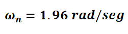
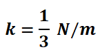 Regresando a la expresión para la frecuencia natural:
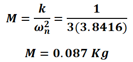 Por último,

 dademuchconnection