
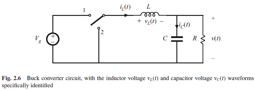
Let us more closely examine the inductor and capacitor waveforms in the buck converter illustrated in Figure 2-6.
In practice, it is impossible to build a perfect low-pass filter that completely removes the AC components at the switching frequencies and its harmonics. So, the low-pass filter must allow at least some small amount of the high-frequencies harmonics generated by the switch to reach the output voltage. Actually, the output voltage appears as illustrated in Figure 2-7.
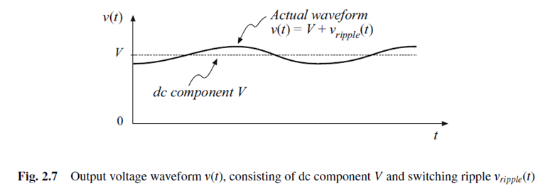
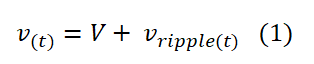
So, the actual output voltage v(t) consists of the desired DC component V, plus a small undesired AC component vripple(t) arising from the incomplete attenuation of the switching harmonics by the low-pass filter. However, the magnitude of vripple(t) has been exaggerated in Figure 2-7. It is nearly always a good approximation to assume that the magnitude of vripple(t) is much smaller than the DC component V:
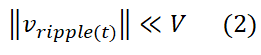
Therefore, output voltage v(t) is well approximated by is DC component V:
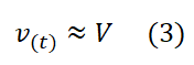
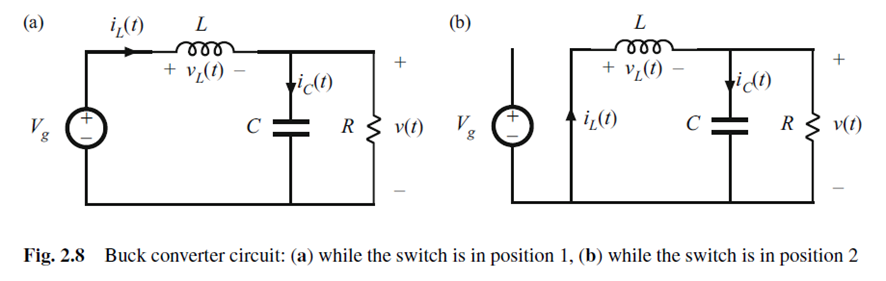
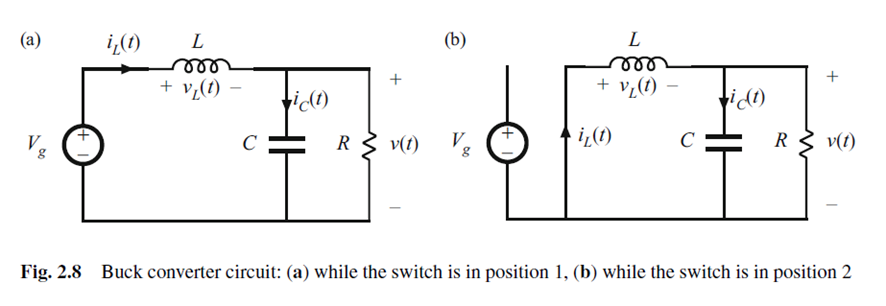
This approximation is known as The small ripple approximation or the linear ripple approximation. With this approximation, we replace the exponential or damped sinusoidal expressions for the inductor and capacitor waveforms with simpler linear waveforms. This approximation is justified provided that the switching period is shorter than the natural time constants of the circuit. Also, this approximation must be applied just to continuous variables: the inductor current and the capacitor voltage. Not to switching voltage, switching current of inductor voltage. Next, let us analyze the inductor current waveform. With the switch in position 1, the circuit reduces to Figure 2.8a.
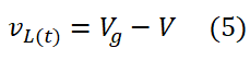
The inductor voltage vL(t) is given by:

Applying small ripple approximation to equation (3):
The inductor current can be found by use of the definition:
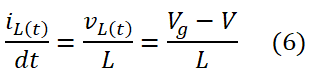
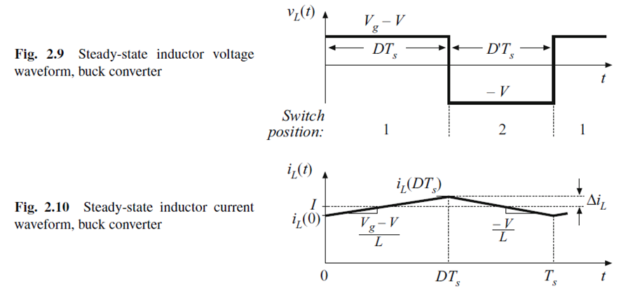
Since the inductor voltage is essentially constant during the first interval (switch in position 1), the inductor current slope of equation (6) is also essentially constant and the inductor current increase linearly, as in Figure 2-10, where we can see vL(t) vs iL(t):
Similar arguments apply in the second interval (switch in position 2). The left side of the inductor is connected to ground, leading to the circuit of Figure 2.8b.
Using the small-ripple approximation leads to:

So:
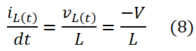
Consequently, during the second interval the inductor current decrease linearly at a constant slope equation (8), as in Figure 2-10 position 2 of the switch.
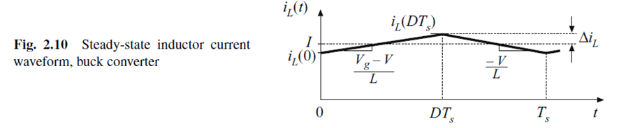
In Figure 2-10 the inductor current iL(t) is symmetrical about I. Since:

is the peak ripple, the peak to peak ripple is:

Which is also the change in current . It is equal to the slope times the length of the first interval DTs:
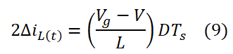
Solution for the peak ripple yields:
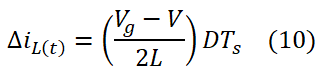
Typical values of the peak ripple lie in the range of 10%-20% of the full-load value of the DC component I. So, by design, the inductor current ripple is also usually small compared to the DC component I. The small approximation is justified:
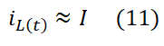
Solution for L in equation (10) yields:
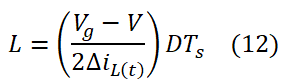
Equation (12) is commonly used to select the value of the inductance at the design of the buck converter. Equations (1) to (12) are derived from steady-state conditions. Source:
- Erickson R., Maksimovic D. Fundamentals of Power Electronics. Pp18-22.
Previously: The Buck Converter (Introduction)
Next: The inductor volt-second balance – Chapter three
Literature review by Larry Obando – Electrical Engineering
Universidad Simón Bolívar – Universidad Central de Venezuela
Mathematical modeling and simulation services
Contacto – Whatsapp +34633129287
dademuchconnection@gmail.com

