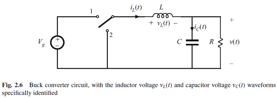
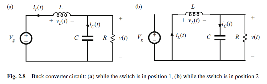
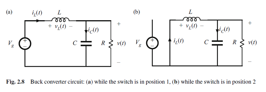
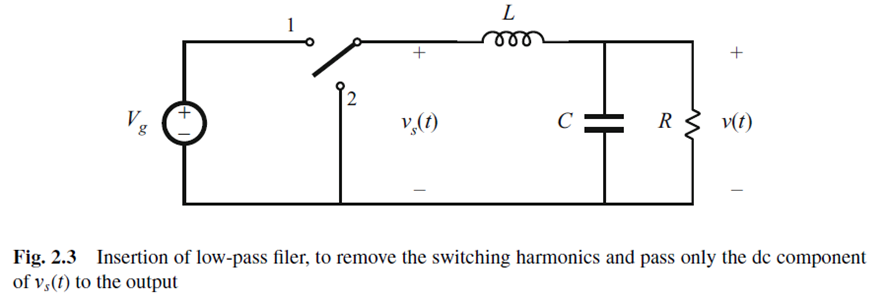
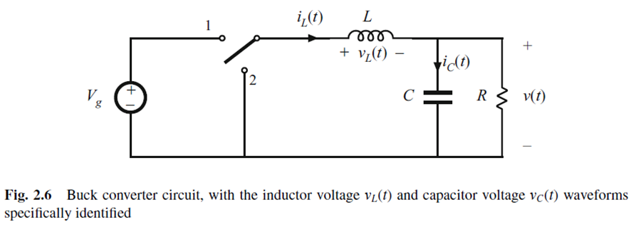
Let us more closely examine the inductor and capacitor waveforms in the buck converter illustrated in Figure 2-6.
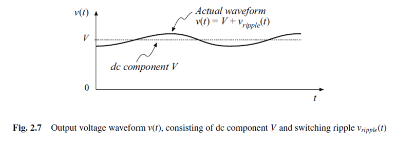
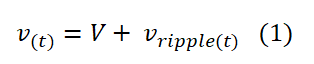
Actually, the output voltage appears as illustrated in Figure 2-7.
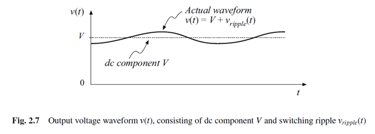
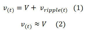
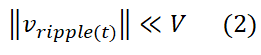
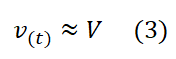
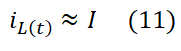
This approximation is known as The small ripple approximation or the linear ripple approximation.
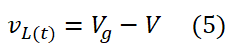
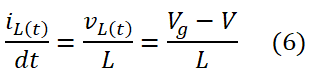
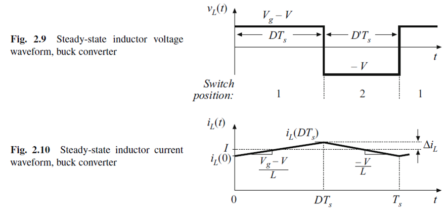
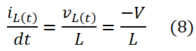
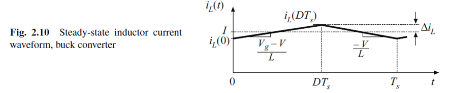
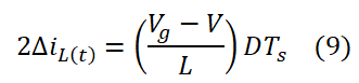
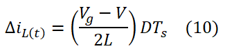
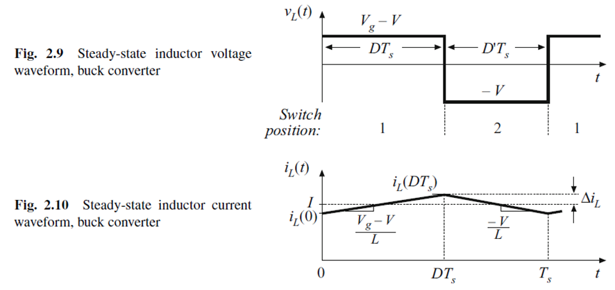
With this approximation, let us analyze the inductor current waveform. Since the inductor voltage is essentially constant during the first interval (switch in position 1), the inductor current slope of equation (6) is also essentially constant and the inductor current increase linearly, as in Figure 2-10:
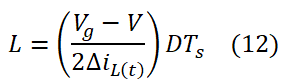
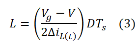
Solution for L yields:
Equations (1) to (3) and Figure 2.10 are derived under steady-state conditions. Let us consider next what happens to the inductor current when the converter is first turned on. Suppose that the inductor current and output voltage are initially zero, and an input voltage Vg is the applied. As shown in Figure 2.11, during the first subinterval, with the switch position in 1, we know that the inductor current will increase.
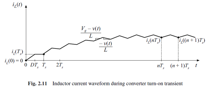
Since the inductor current iL(t) flows to the output, the output capacitor will charge slightly, and will v(t) increase slightly too. The process repeats during the second and succeeding switching periods, with inductor current iL(t) increasing during each subinterval 1 and decreasing during each subinterval 2.
As the output capacitor continues to charge and v(t) increases, the slope during each subinterval 1 decreases and the slope during each subinterval 2 becomes more negative. There is no change in the inductor current over a complete switching period and the converter reachs the steady state condition.
The requirement that, in equilibrium, the net change in inductor current over one switching period be zero lead us to a way to find steady-state condition in any switching converter. That is what we call the inductor volt-second balance.
Given the defining relation of an inductor:
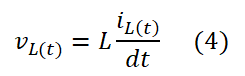
Integration over one complete switching period, say from t=0 to t=Ts yields:
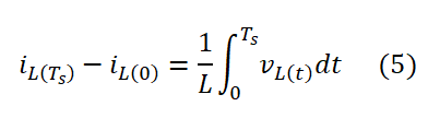
In steady-state condition, the initial and final value of the inductor current is equal, so:
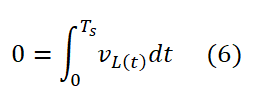
The right hand of equation (6) has the units of volt-second or flux-linkages. It states that the total area, or net volt-seconds, under the vL(t) waveform must be zero under steady-state condition.
An equivalent form is obtained by dividing both sides of equation (6) by the switching period:
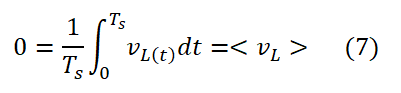
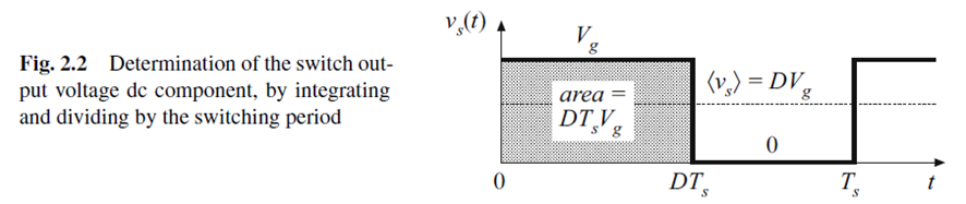
Equation (7) is recognized as the average value, or DC component, of vL(t). Equation (7) states that, under steady-state condition, the applied inductor voltage must have zero DC component.
The inductor voltage waveform is reproduced in Figure 2.12 with the area, or net volt-seconds, under the vL(t) curve identified.
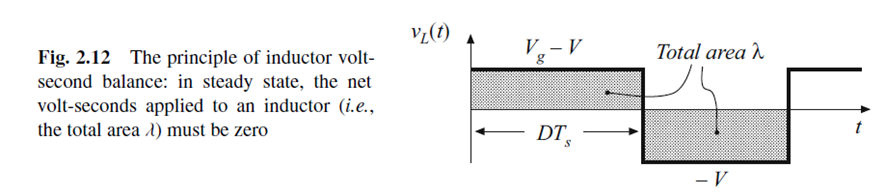
The total area lambda is given by the areas of the two rectangles:

The average value is therefore:

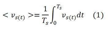
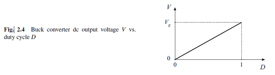
What lead us to state, using equation (2), that:
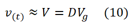
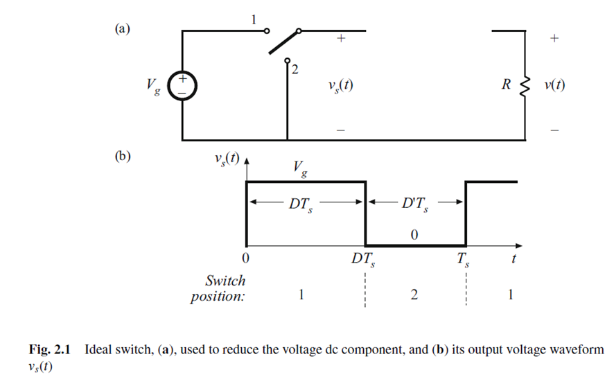
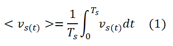
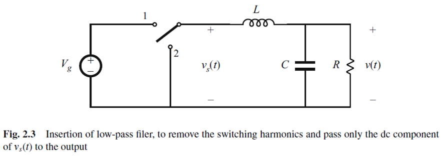
Considering Figure 2.3, the output voltage v(t) of a Buck Converter is essentially equal to the DC component of the switching voltage vs(t), and equation (10) states that the output voltage v(t) is less than or equal to the input voltage Vg, since 0<D<1.
Source:
- Erickson R., Maksimovic D. Fundamentals of Power Electronics. Pp. 22-24.
Previously: The small ripple approximation – Chapter two
Literature review by Larry Obando – Electrical Engineering
Universidad Simón Bolívar – Universidad Central de Venezuela
Mathematical modeling and simulation services
Contacto – Whatsapp +34633129287
dademuchconnection@gmail.com