Effects of the addition of zeros: the addition of a zero to the open loop transfer function has the effect of pulling the rootlocus to the left, with which the system tends to be more stable, and also accelerates the settlement of the response. The effect of such control is to introduce a degree of foresight to the system and speed up the transient response.
To illustrate this effect, let’s look at the following example:
Example 1
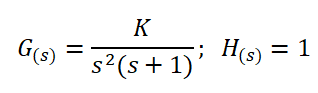
Suppose we are in the presence of a system with an unstable plant. An example of such a situation is the following:
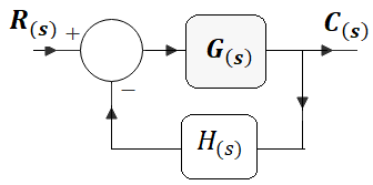
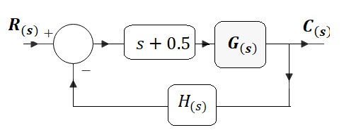
Where G (s) is the transfer function of the plant and H (s) is the transfer function of the sensor used to assemble the closed-loop system, as shown in Figure 1:
Figure 1
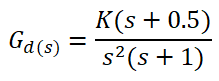
We know from Block Algebra and Transfer Function theory that the open loop transfer function of this system Gd (s) is:
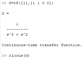
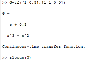
We also know that the rootlocus is drawn with the open loop transfer function of this system Gd (s), for which we can use the following command in Matlab:
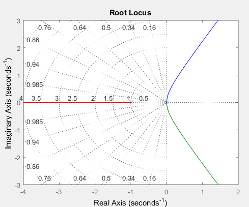
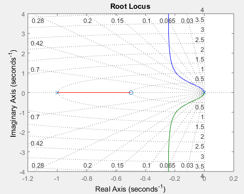
Graph 1
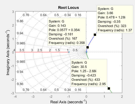
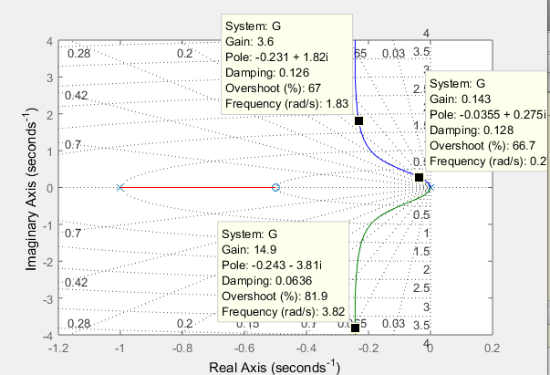
Analysis: In graph 1 we can see that the system is unstable for all positive values of gain K. That is, if we move through the blue and green curves, varying the value of K, as in graph 2, where K1 = 0.143; K2 = 3.66 and K1 = 30.5, respectively, we see that the poles of the system are located on the right side of the s-plane, and therefore it is an unstable system:
Let’s apply the principle of addition of a zero to the open loop transfer function for this case. We are going to add a zero at s = -0.5 (Figure 2), therefore the Gd (s) of the system is:
Figure 2
Let’s see the effect of adding a zero to the system by:
Graph 3
Analysis: In graph 3 we see that the LGR of the system has shifted to the left and that the system is stable for any positive value of the gain k, that is, that all the poles of the closed-loop system are located on the left side from plane s (Graph 4), an essential condition for the system to be stable:
Graph 4
Source:
Katsuhiko Ogata, Modern Control Engineering, pages 442-443.
Written by: Larry Francis Obando – Technical Specialist – Educational Content Writer.
We discuss two ways to improve the steady-state error of a feedback control system using cascade compensation. One objective of this design is to improve the steady-state error without appreciably affecting the transient response.
Improving Transient Response - Compensation
We have seen before that setting the gain at a particular value on the root locus yields the transient response dictated by the poles at that point on the root locus. Thus, we are limited to those responses that exist along the root locus. (See Sketching Root Locus with Matlab – Control Systems)
Unfortunately, most of the time the overshoot specification for designing control systems exceed the posibilities of the current root locus. What can we do then?
Rather than change the existing system, we augment, or compensate, the system with additional poles and zeros, so that the compensated system has a root locus that goes through the desired pole location for some value of gain. One of the advantages of compensating a system in this way is that additional poles and zeros can be added at the low-power end of the system before the plant. We should evaluate the transient response through simulation after the design is complete to be sure the requirements have been met.
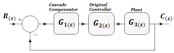
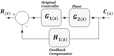
There are two configurations of compensation mostly used in control systems design: cascade compensation and feedback compensation. These methods are modeled in Figure 1 and Figure 2:
Figure 1. Cascade Compensation of a control system.
With cascade compensation, the compensating network, G1(s), is placed at the low-power end of the forward path in cascade with the plant, Figure 1.
Figure 2. Feedback Compensation of a control system.
With feedback compensation, the compensator, H1(s), is placed in the feedback path, Figure 2.
Both methods change the open-loop poles and zeros, thereby creating a new root locus that goes through the desired closed-loop pole location.
Cascade Compensation - PI Controller
Steady-state error can be improved by placing an open-loop pole at the origin,
because this increases the system type by one. For example, a Type 0 system
responding to a step input with a finite error, will responds with zero error if the system
type is increased by one. But, we want to do this without affecting the transient response.
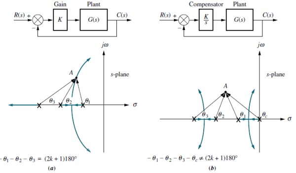
However, if we add a pole at the origin to increase the system type, the angular contribution of the open-loop poles at hypothetical point A is no longer 180, and the root locus no longer goes through point A, as shown in Figure 3.a and 3.b:
Figure 3.
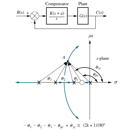
To solve the problem, we also add a zero close to the pole at the origin, as shown
in Figure 4:
Figure 4.
Now the angular contribution of the compensator zero and compensator pole cancel out, point A is still on the root locus, and the system type has been increased. That is how we can improve the steady-state error without affecting the transient response.
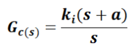
A compensator with a pole at the origin and a zero close to the pole is called an ideal integral compensator, or Proportional-plus-Integral PI compensator, which transfer function Gc(s) is:
Next example allows to find how PI compensation works.
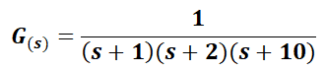
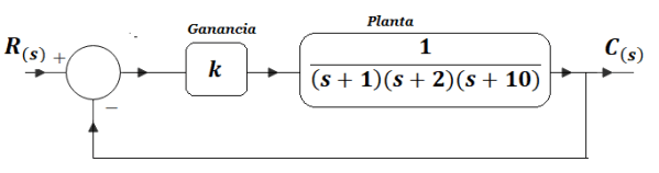
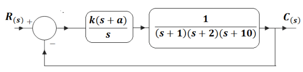
For control system of Figure 5, it is required to reduce steady-state error to zero, through a PI controller, keeping damping at ξ=0.173. The plant transfer function is G(s) and its original controller is represented by the gain k:
Figure 5.
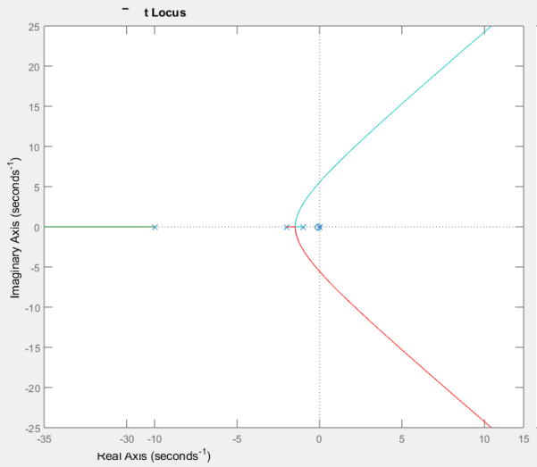
The first step is to evaluate the system before the compensation, then to find the location of the two closed-loop second-order dominant poles in order to get the damping requiered by the design specifications.
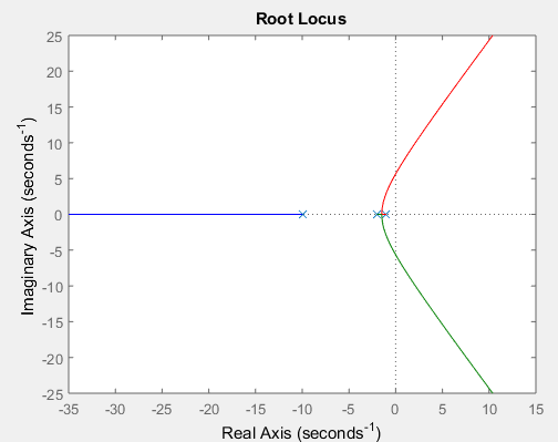
Figure 6 shows the Root-Locus of the system before compensation:
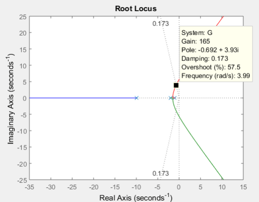
Using the damping line in Matlab, we can find the intersection point between the root-locus and the value ξ=0.173, as we can see in Figure 7:
>> z=0.173;
>> sgrid(z,0)
Figure 7.
The intersection of Figure 7 shows us that adjusting the gain to k=165 of the original controller, we obtain the damping requiered: ξ=0.173. We also see in Figure 7 that the closed-loop second-order dominant poles s1 and s2, before compensation are:
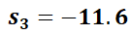
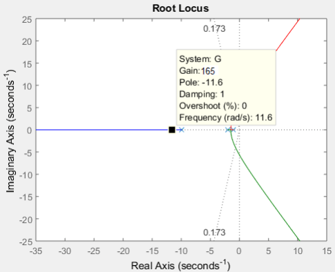
Now we look for the third pole in the root locus. In Figure 8 we must set the same gain k=165 at the third pole line, in consequence s3 is located at:
Figure 8.
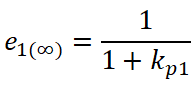
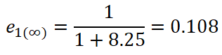
With k=165 we calculate the steady-state error e1(∞) for a step input, before compensation:
Where kp1 the position constant before compensation:
Where kG(s) is the system forward transfer function multiplied by the adjusted gain, before compensation, as in Figure 5. Therefore:
We add a PI controller in cascade into the system, as in Figure 9:
Figure 9.
Here, we have matched the gain constant of the compensator with the original gain constant, that is to say k=ki. The constant a is determined by the location of compensator zero, wich must be near the compensator pole. That is why we set the compensator zero at s=-0.1 , that is to say a=0.1. The root locus of this compensated system is in Figure 10:
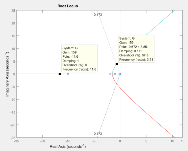
In view of the fact that we want to maintain the transient response as unchanged as possible, in Figure 11 we draw the damping line in the root locus and search for the point of intersection between the lines of the root locus and ξ=0.173:
>> z=0.173;
>> sgrid(z,0);
Figure 11.
Adjusting the gain to k=159 in Figure 11, we obtain the damping ξ=0.173. We see that closed-loop second-order dominant poles s1 and s2, after compensation, are:
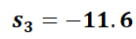
Looking for the third pole in the root locus, we must set the gain k=159 at the third pole line. After that, s3 is located at:
These results show that approximately the values of the 3 poles before and after the PI compensation have been conserved, indicating a similar transient response after correcting the error in steady state from 0.108 to 0, as shwon later.
The forward transfer function G2(s) of the system after compensation is:
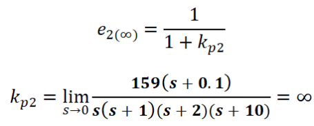
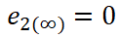
One more time, we calculate steady-state error e2(∞) for a step input, after compensation:
In consequence:
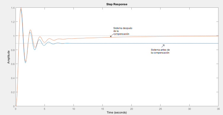
Figure 12 compares the step response of the closed-loop system before and after compensatio PI:
Figure 12 shows that through PI compensation we have managed to improve the steady-state error without considerably modifying the transient response of the original system.
Compensación en Cascada - Lag Compensation
In construction…
Source :
Control Systems Engineering, Nise
Written by Prof. Larry Francis Obando – Technical Specialist – Educational Content Writer
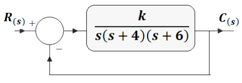
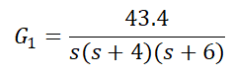
Given the system of Figure 1, design a PD compensator to yield a 16% overshoot, with a threefold reduction in settling time (one-third of the uncompensated system’s settling time).
Figure 1
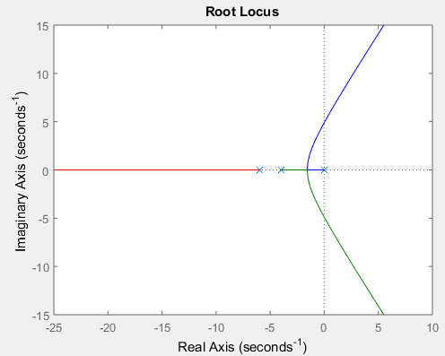
Let us first evaluate the performance of the uncompensated system. The root locus for the uncompensated system is shown in Figure 2:
>> s=tf(‘s’);
>> G=1/(s*(s+4)*(s+6));
Figure 2
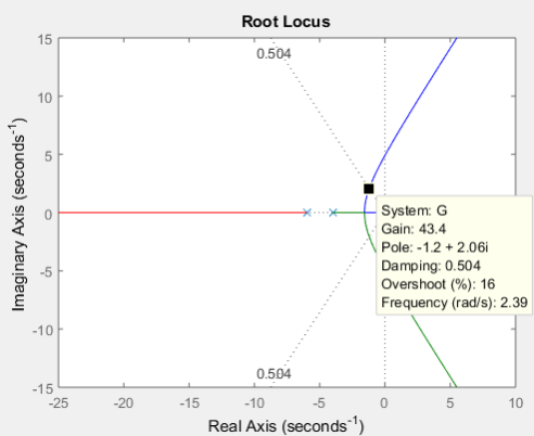
Since 16% overshoot is equivalent to ξ=0.504, we search along that damping ratio line in Figure 3:
>> z=0.504;
>> sgrid(z,0);
Figure 3
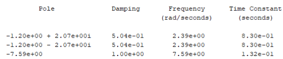
According to Figure 3, adjusting the gain to k=43.4 we get ξ=0.504 and a natural frequency ω=2.39 rad/s.
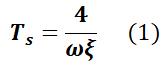
Based upon a second-order approximation, we can use the 2% criteria and calculate the settling-time Ts1before the compensation, as a function of the naural frequency ω and the damping ξ, by means of the following equation:
Simulation of Figure 3 generates the necessary values for equation (1), so that:
In the other hand, the value of the factor ω*ξ=1.2045 matches the real part σ of closed-loop second-order dominant poles, as we can see in Figure 3 or by the following command in Matlab, taking into consideration that the straight-forward transfer function is now G1:
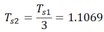
The desig requirements ask for an 16% overshoot and a reduction of the settling-time of 1/3 after compensation. So, the settling-time Ts2after compensation is:
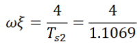
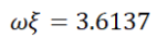
Using equation (1) we can know the value of the factor ω*ξ after compensation:
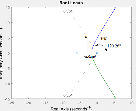
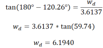
That is to say, the real part of second-order dominant poles after compensation is σ=3.6137. To find the imaginary part wd we use the root-locus of Figure 4:
Figure 4.
Consequently, after compensation the second-order dominant poles must be located at p=-3.6137+j6.1940.
Now, to evaluate the whole system we will use point p as a test point.
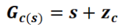
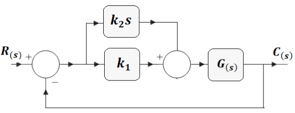
PD compensation consists of a cascaded controller with a Gc(s) transfer funcion that is:
The configuration of such a controller is:
Figure 5.
Next step is to design the location of Zero zc using the test point p and finding the equivalent values for k1and k2.
The result is the sum of the angles to the design point of all the poles and zeros of the compensated system except for those of the compensator zero itself. The difference between the result obtained and 180 is the angular contribution required of the compensator zc es:
The geometry is shown in Figura 6, where we can get the real part of zc by means of the following formula:
Figure 6.
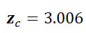
From where:
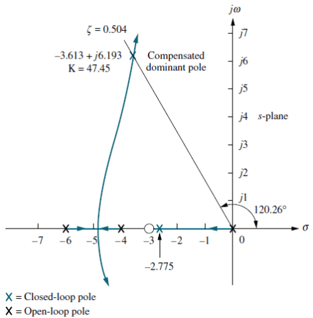
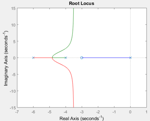
Now, we study the root-locus of Figure 7, where the forward-path transfer function is G2:
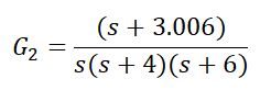
>> G2=(s+3.006)/(s*(s+4)*(s+6));
>> rlocus(G2)
Figure 7.
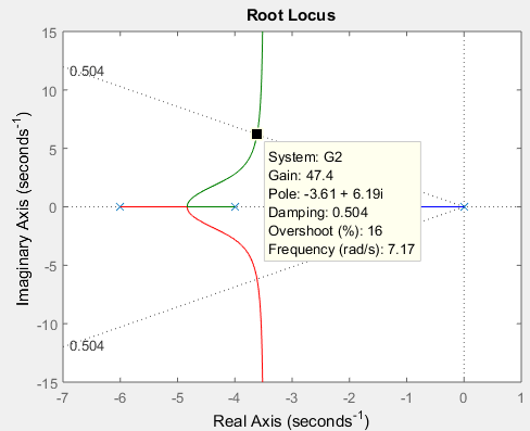
According to Figure 8, adjusting the gain k=47.4 we keep ξ=0.504, an overshoot16%, the second-order dominant pole s=-3.6137+j6.1940, at a natural frequency ω=7.17 rad/s.
>> z=0.504;
>> sgrid(z,0);
Figure 8.
With this new data, we evaluate the settling-time Ts2 after compensation:
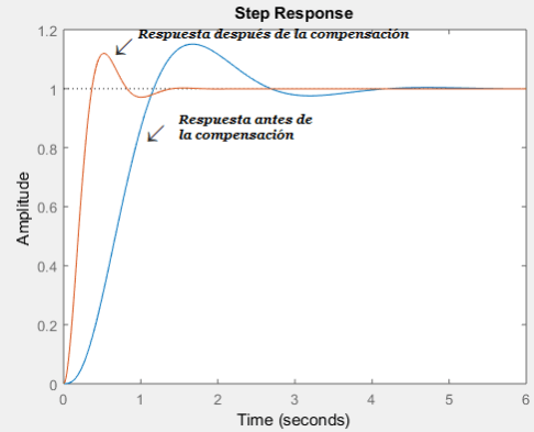
It shows that we have achieved the design goal. Figure 9 compares the response of the closed-loop system to an step input before and after PD compensation:
The response of Figure 9 shows a considerable improvement in the settling-time and, in general, the compensation allows a faster system with an overshoot that does not vary much. Before compensation, Ts=3.4712 s. After compensation, Ts=1.1527 s.
An alternative design process in Matlab
Use MATLAB, the Control System Toobox, and the following steps to use SISOTOOL to perform the design of last Example.
Type sisotool in the MATLAB Command Window.
Select Import in the File menu of the SISO Design for SISO Design Task Window.
In the Data field for G, type zpk([],[0,-4,-6],1) and hit ENTER on the keyboard. Click OK.
On the Edit menu choose SISO Tool Preferences . . . and select Zero/pole/gain: under the Options tab. Click OK.
Right-click on the root locus white space and choose Design Requirements/New . . .
Choose Percent overshoot and type in 16. Click OK.
Right-click on the root locus white space and choose Design Requirements/New . . .
Choose Settling time and click OK.
Drag the settling time vertical line to the intersection of the root locus and 16%
overshoot radial line.
Read the settling time at the bottom of the window.
Drag the settling time vertical line to a settling time that is 1/3 of the value
found in Step 9.
Click on a red zero icon in the menu bar. Place the zero on the root locus real axis by clicking again on the real axis.
Left-click on the real-axis zero and drag it along the real axis until the root locus intersects the settling time and percent overshoot lines.
Drag a red square along the root locus until it is at the intersection of the root locus,
settling time line, and the percent overshoot line.
Click the Compensator Editor tab of the Control and Estimation Tools Manager window to see the resulting compensator, including the gain.
Source:
Control Systems Engineering, Nise
Written by: Larry Francis Obando – Technical Specialist – Educational Content Writer.
Mentoring Académico / Empresarial / Emprendedores
Copywriting, Content Marketing, Tesis, Monografías, Paper Académicos, White Papers (Español – Inglés)
Escuela de Ingeniería Eléctrica de la Universidad Central de Venezuela, Caracas.
Escuela de Ingeniería Electrónica de la Universidad Simón Bolívar, Valle de Sartenejas.
Escuela de Turismo de la Universidad Simón Bolívar, Núcleo Litoral.
NEXT: PID – Effect of integrative and derivative control actions.
Introduction
An automatic controller compares the real value of the output of a plant with the input reference (the desired value), determines the deviation and produces a control signal that will reduce the deviation to zero or a small value. The way in which the automatic controller produces the control signal is called control action.
Classification of industrial controls
According to their control actions, industrial controllers are classified as:
Two-position (On / Off)
Proportional
Integrals
Proportional-Integrals
Proportional-Derivatives
Proportional-Integrals-Derivatives
Almost all industrial controllers use electricity as an energy source or a pressurized fluid, such as oil or air. The controllers can also be classified, according to the type of energy they use in their operation, like pneumatic, hydraulic or electronic. The type of controller that is used must be decided based on the nature of the plant and operational conditions, including considerations such as safety, cost, availability, reliability, precision, weight and size.
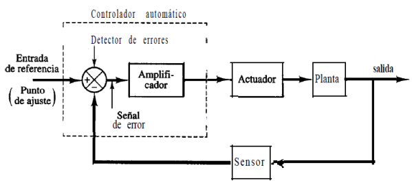
Figure 5-1 shows a typical configuration for an Industrial Control System:
The previous figure consists of a Block Diagram for an industrial control system composed of an automatic controller, an actuator, a plant and a sensor (measuring element). The controller detects the error signal, which is usually at a very low power level, and amplifies it to a sufficiently high level. The output of an automatic controller feeds an actuator that can be a pneumatic valve or an electric motor. The actuator is a power device that produces the input for The plant according to the control signal, so that the output signal approaches the reference input signal. The sensor, or measurement element, is a device that converts an output variable, such as a displacement, into another manageable variable, such as a voltage, that can be used to compare the output with the reference input signal. This element is in the feedback path of the closed-loop system. The setpoint of the controller must be converted into a reference input with the same units as the feedback signal from the sensor or from the measuring element.
Two positions control (On / Off).
In a two position control system, the acting element only has two fixed positions that, in many cases, are simply turned on and off. The On/Off control is relatively simple and cheap, which is why it is extensively used in industrial and domestic control systems.
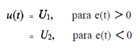
Suppose that the output signal of the controller is u(t) and that the error signal is e(t). In the control of two positions, the signal u(t) remains at a value either maximum or minimum, depending on whether the error signal is positive or negative. In this way,
where U1 y U2 are constants. Very often, the minimum value of U2 is zero or –U1.
It is common for two-position controllers to be electrical devices, in which case an electrical valve operated by solenoids is widely used. Pneumatic proportional controllers with very high gains function as two-position controllers and are sometimes referred to as two-position pneumatic controllers.
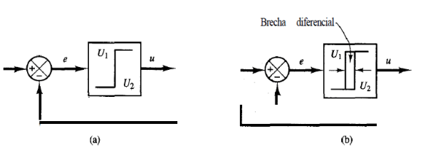
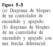
Figures 5-3 (a) and (b) show the block diagrams for two controllers of two positions The range in which the error signal must move before the commutation is called differential gap. In Figure 5-3 (b) a differential gap is indicated. Such a gap causes the output of the controller u (t) to retain its present value until the error signal has moved slightly beyond zero. In some cases, the differential gap is the result of unintentional friction and a lost movement; however, it is often intentionally caused to avoid too frequent operation of the on and off mechanism.
Proportional control action.
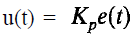
For a controller with proportional control action, the relationship between the controller output u (t) and the error signal e (t) is:
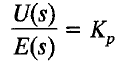
or, in quantities transformed by the Laplace method:
where Kp is considered proportional gain.
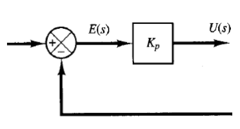
Whatever the actual mechanism and the form of the operating power, the controller
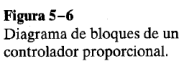
proportional is, in essence, an amplifier with an adjustable gain. A block diagram of such a controller is presented in Figure 5-6.
Integral control action.
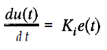
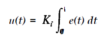
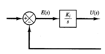
In a controller with integral control action, the value of the controller output u (t) is changed to a ratio proportional to the error signal e (t). That is to say,
O well:
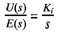
where Ki is an adjustable constant. The transfer function of the integral controller is:
If the value of e (t) is doubled, the value of u (t) varies twice as fast. For an error of zero, the value of u (t) remains stationary. Sometimes, the integral control action is called adjustment control (reset). Figure 5-7 shows a block diagram of such controller.
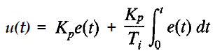
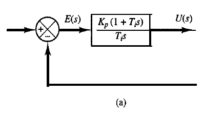
Integral-proportional control action. The control action of a proportional-integral controller (PI) is defined by:
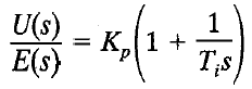
or the transfer function of the controller, which is:
where Kp is the proportional gain and Ti is called integral time. Both Kp and Ti are adjustable. Integral time adjusts the integral control action, while a change in the value of Kp affects the integral and proportional parts of the control action.
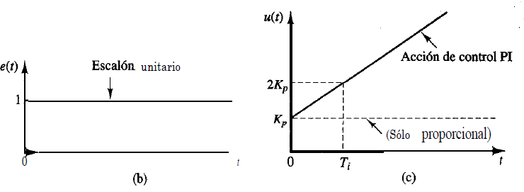
The inverse of the integral time Ti is called the readjustment speed. The rate of readjustment is the number of times per minute that the proportional part of the control action is doubled. The rate of readjustment is measured in terms of the repetitions per minute. The Figure 5-8 (a) shows a block diagram of a PI controller. If the error signal e (t) is a unit step function, as shown in Figure 5-8 (b), the controller output u (t) becomes what is shown in Figure 5-8 (c).
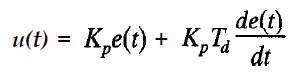
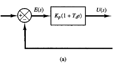
Proportional-derivative control action. The control action of a proportional-derivative (PD) controller is defined by:
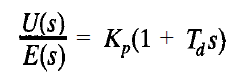
The transfer function is:
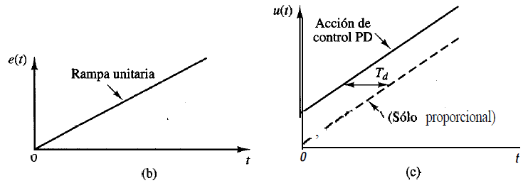
where Kp is the proportional gain and Td is a constant called derivative time. Both Kp and Td are adjustable. The derivative control action, sometimes called speed control, occurs where the magnitude of the controller output is proportional to the rate of change of the error signal. The derivative time Td is the time interval during which the action of the velocity advances the effect of the proportional control action.
Figure 5-9 (a) shows a block diagram of a PD controller. If the error signal e (t) is a unit ramp function as shown in Figure 5-9 (b), the controller output u (t) becomes that shown in Figure 5-9 (c). ). The derivative control action has a forecast nature. However, it is obvious that a derivative control action never foresees an action that has never occurred.
Although the derivative control action has the advantage of being forecast, it has the disadvantages that it amplifies the noise signals and can cause a saturation effect in the actuator. Note that the derivative control action is never used alone, because it is only effective during transient periods.
Proportional-Integral-derivative (PID) control action.
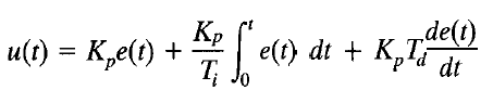
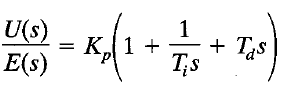
The combination of a proportional control action, an integral control action and a derivative control action is called proportional-integral-derivative (PID) control action.
This combined action has the advantages of each of the three individual control actions. The equation of a controller with this combined action is obtained by:
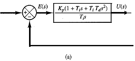
The transfer function is:
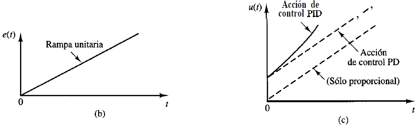
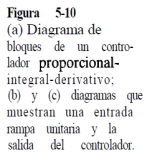
where Kp is the proportional gain, Ti is the integral time and Td is the derivative time. The block diagram of a PID controller appears in Figure 5-10 (a). If e (t) is a unit ramp function, like the one shown in Fig. 5-10 (b), the controller output u (t) becomes that of Fig. 5-10 (c).
Effects of the sensor on the performance of the system.
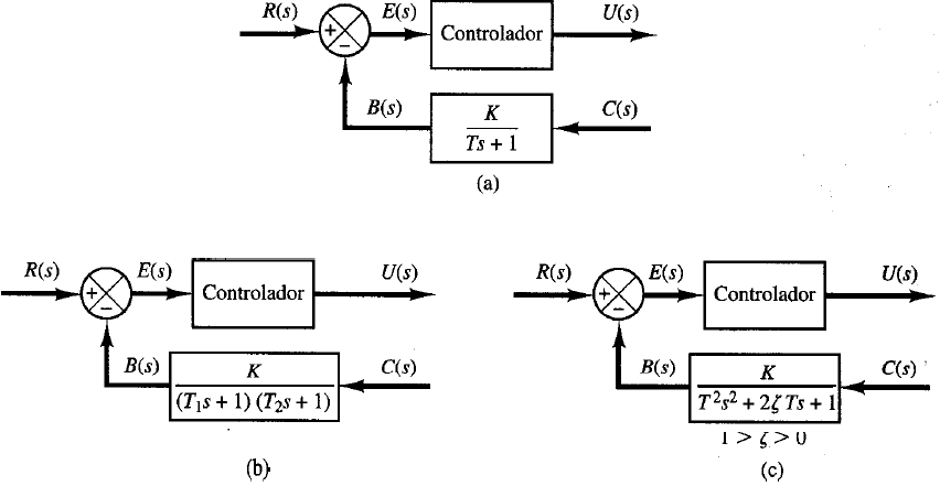
Since the dynamic and static characteristics of the sensor or measuring element affects the indication of the actual value of the output variable, the sensor fulfills a function important to determine the overall performance of the control system. As usual, the sensor determines the transfer function in the feedback path. If the time constants of a sensor are negligible compared to other constants of time of the control system, the sensor transfer function simply it becomes a constant. Figures 5-11 (a), (b) and (c) show diagrams of automatic controller blocks with a first-order sensor, an overdamped second-order sensor and a second-order underdamped sensor, respectively. Often the response of a thermal sensor is of the overdamped second order type.