Sin categoría

Medicina Lifestyle – Definición y alcance

Lifestyle Medicine es la ciencia y la aplicación de estilos de vida saludables que intervienen para la prevención y el tratamiento de enfermedades relacionadas con el estilo de vida, como enfermedades cardíacas, diabetes, derrames cerebrales, obesidad, algunas afecciones neurológicas y algunos tipos de cáncer. Es la especialidad basada en la evidencia que une la ciencia de la actividad física, la nutrición, el manejo del estrés y la resiliencia, la higiene del sueño y otros hábitos saludables para los individuos a través de la práctica clínica en cuidado de la salud.

El mejor secreto de la medicina es el poder de la nutrición, cuando el cuerpo se cura a sí mismo. Esta es la mejor inversión que una persona puede hacer. (The Best Kept Secret in Medicine).
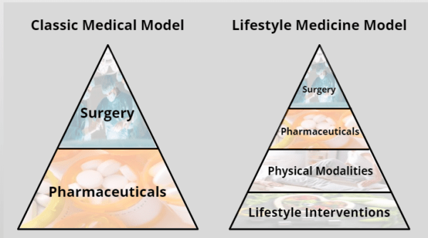
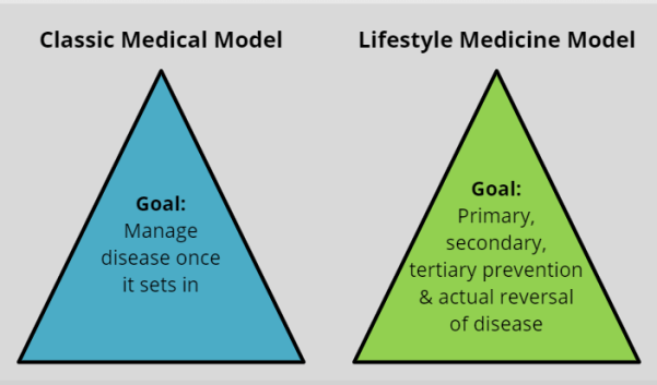
La intervención en el estilo de vida (Lifestyle intervention) es un elemento clave de la prevención y el control de la hipertensión, la insuficiencia cardíaca, las enfermedades cardiovasculares, los accidentes cerebrovasculares, el cáncer, la diabetes y la muerte por todas las causas. Esto porque reduce la presión arterial, la glucosa, el colesterol e influye en las causas fundamentales y los mecanismos biológicos que conducen a la enfermedad. Por ejemplo, en un estudio sobre la salud de las enfermeras se encontró que el riesgo de enfermedad coronaria 15 y diabetes mellitus tipo 216 se redujo 5 y 10 veces, respectivamente, entre los que participaron en 5 comportamientos saludables modificables.

Cuadro comparativo:

Los resultados del siguiente estudio nacional realizado en el año 2000: Healthy_lifestyle_characteristics_2000, muestran que solo el 3.0% de los adultos de EE. UU. siguieron una combinación de 4 características de estilo de vida modificables: no fumar, peso saludable, consumo adecuado de frutas y verduras, y actividad física regular. Ningún subgrupo se involucró en los 4 estilos de vida saludables en ningún grado importante; el predominio más alto es solo del 5.7%. Estos resultados ilustran el extraordinariamente bajo predominio de estilos de vida saludables en la población adulta de EE. UU.

En la Tabla 2 se muestran las estimaciones de predominio ajustadas por edad del indicador de estilo de vida saludable (es decir, la participación en las 4 Healthy Lifestyle Characteristics or HLCs for short) según las 6 variables demográficas y relacionadas con la salud.

El predominio general fue de solo el 3.0% y las diferencias absolutas entre los subgrupos fueron pequeñas, con un rango desde el 0.8% (en personas con educación inferior a la secundaria) hasta solo el 5.7% (en personas con excelente salud):

Los objetivos de este estudio fueron informar sobre el predominio de las características del estilo de vida saludable (HLCs) y generar un indicador único de un estilo de vida saludable.

Definimos los siguientes 4 HLCs: no fumador; peso saludable (índice de masa corporal [calculado como peso en kilogramos dividido por el cuadrado de la altura en metros] de 18.5-25.0); consumir 5 o más frutas y verduras por día; y actividad física regular (30 minutos por 5 veces por semana).

Las 4 HLCs se sumaron para crear un índice de estilo de vida saludable (rango, 0-4), y el patrón de seguimiento de las 4 HLCs se definió como un único indicador de estilo de vida saludable.

Al utilizar datos de más de 153 000 adultos, el predominio (intervalo de confianza del 95%) de las HLCs individuales fue la siguiente: no fumadores, 76.0% (75.6% -76.4%); peso saludable, 40.1% (39.7% -40.5%); 5 frutas y verduras por día, 23.3% (22.9% -23.7%); y actividad física regular, 22.2% (21.8% -22.6%). El predominio general del indicador de estilo de vida saludable (es decir, que tiene las 4 HLCs) fue de solo el 3,0% (intervalo de confianza del 95%, 2,8% -3,2%), con poca variación entre los subgrupos (rango, 0,8% -5,7%).

Conclusión: estos datos ilustran que muy pocos adultos en los Estados Unidos llevan a cabo un estilo de vida saludable, definido como una combinación de 4 HLCs, y que ningún subgrupo siguió esta combinación a un nivel remotamente compatible con las recomendaciones clínicas o de salud pública.

Las estimaciones de predominio de cada HLCs según las 6 variables demográficas y relacionadas con la salud se muestran en la Tabla 1:
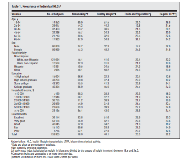
El setenta y seis por ciento (95% CI, 75.6% -76.4%) de los adultos de EE. UU. no fuma cigarrillos actualmente. Esta tendencia se mostró fuertemente positiva al aumentar la edad, la educación, los ingresos familiares y el estado de salud. Solo el 40,1% (95% CI, 39,7-40,5%) de los adultos tenía peso saludable, que mostró una fuerte tendencia inversa con la edad y tendencias positivas con la educación y el estado de salud. El peso saludable fue más común en las mujeres y entre los blancos. Solo el 23.3% (95% CI, 22.9% -23.7%) de las personas consumió frutas y verduras 5 o más veces por día, mientras que el LTPA (Leisure Time Physical Activity) regular se realizó en solo 22.2% (95% CI, 21.8% -22.6%).

Comentarios:

Los resultados generados a partir de esta base de datos representativa a nivel nacional indican que solo el 3.0% de los adultos de EE. UU. siguieron una combinación de 4 características de estilo de vida modificables: no fumar, peso saludable, consumo adecuado de frutas y verduras, y actividad física regular. Ningún subgrupo se involucró en los 4 estilos de vida saludables en ningún grado importante; el predominio más alto fue de solo el 5.7%. Estos resultados ilustran el extraordinariamente bajo predominio de los estilos de vida saludables en la población adulta de EE. UU.
Revisión Bibliográfica:

Date: February 2019, Location: Caracas, Quito, Guayaquil.

Fuentes:

  1. Introduction to Lifestyle MedicineIn Module 1, you will be able to:

Escrito por Prof. Larry Francis Obando – Technical Specialist – Educational Content Writer

Mentoring Académico / Emprendedores / Empresarial

Copywriting, Content Marketing, Tesis, Monografías, Paper Académicos, White Papers (Español – Inglés)

Escuela de Ingeniería Eléctrica de la Universidad Central de Venezuela, UCV CCs

Escuela de Ingeniería Electrónica de la Universidad Simón Bolívar, USB Valle de Sartenejas.

Escuela de Turismo de la Universidad Simón Bolívar, Núcleo Litoral.

Contact: Caracas, Quito, Guayaquil, Cuenca. telf – 0998524011

WhatsApp: +593981478463

email: dademuchconnection@gmail.com
Sin categoría

Lifestyle Medicine definition and scope.

Lifestyle Medicine is the science and application of healthy lifestyles as interventions for the prevention and treatment of lifestyle-related diseases such as heart disease, diabetes, stroke, obesity, some neurological conditions and some cancers. It is the evidence-based specialty bridging the science of physical activity, nutrition, stress management and resilience; sleep hygiene and other healthy habits to individuals through clinical practice in healthcare.

The best keep secret in medicine is the power of nutrition, when the body heals himself. This is the best investment you can make (The Best Kept Secret in Medicine).

Lifestyle intervention is a key element of prevention and control of hypertension, heart failure, cardiovascular disease, stroke, cancer, diabetes, and death from all causes. This because it reduces blood pressure, glucose, cholesterol, and influence the fundamental causes and biological mechanisms leading to disease. For example, the Nurses’ Health Study found that the risk of coronary heart disease15 and type 2 diabetes mellitus16 was reduced 5- and 10-fold, respectively, among those who engaged in 5 modifiable healthy behaviors.

Comparative chart:

The results from this nationally representative database 2000 Study: Healthy_lifestyle_characteristics_2000, show that just 3.0% of US adults followed a combination of 4 modifiable lifestyle characteristics— nonsmoking, healthy weight, adequate fruit and vegetable consumption, and regular physical activity. No subgroup engaged in all 4 healthy lifestyles to any important degree— the highest prevalence being only 5.7%. These results illustrate the extraordinarily low prevalence of healthy lifestyles in the US adult population.

The age-adjusted prevalence estimates of the healthy lifestyle indicator (ie, engaging in all 4 HLCs) by the 6 demographic and health-related variables are shown in Table 2.

The overall prevalence was only 3.0%, and the absolute differences across subgroups were small, ranging from 0.8% (in persons with less than high school education) to only 5.7% (in persons in excellent health):

The objectives of this study were to report on the prevalence of healthy lifestyle characteristics (HLCs) and to generate a single indicator of a healthy lifestyle.

We defined the following 4 HLCs: nonsmoking, healthy weight (body mass index [calculated as weight in kilograms divided by the square of height in meters] of 18.5-25.0), consuming 5 or more fruits and vegetables per day, and regular physical activity (30 minutes for5 times per week).

The 4 HLCs were summed to create a healthy lifestyle index (range, 0-4), and the pattern of following all 4 HLCs was defined as a single healthy lifestyle indicator.

By using data from more than 153 000 adults, the prevalence (95% confidence interval) of the individual HLCs was as follows: nonsmoking, 76.0% (75.6%-76.4%); healthy weight, 40.1% (39.7%-40.5%); 5 fruits and vegetables per day, 23.3% (22.9%-23.7%); and regular physical activity, 22.2% (21.8%-22.6%). The overall prevalence of the healthy lifestyle indicator (ie, having all 4 HLCs) was only 3.0% (95% confidence interval, 2.8%-3.2%), with little variation among subgroups (range, 0.8%-5.7%).

Conclusion: These data illustrate that a healthy lifestyle— defined as a combination of 4 HLCs—was undertaken by very few adults in the United States, and that no subgroup followed this combination to a level remotely consistent with clinical or public health recommendations.

The prevalence estimates of each HLC by the 6 demographic and health-related variables are shown in Table1:

Seventy-six percent (95% CI, 75.6%-76.4%) of US adults did not currently smoke cigarettes. Nonsmoking showed strong positive trends with increasing age, education, household income, and health status. Only 40.1% (95% CI, 39.7-40.5%) of adults had healthy weight, which showed a strong inverse trend with age and positive trends with education and health status. Healthy weight was more common in women and among whites. Only 23.3% (95% CI, 22.9%-23.7%) of persons consumed fruits and vegetables 5 or more times per day, while regular LTPA was undertaken by only 22.2% (95% CI, 21.8%-22.6%).

Comments:

The results generated from this nationally representative database indicate that just 3.0% of US adults followed a combination of 4 modifiable lifestyle characteristics— nonsmoking, healthy weight, adequate fruit and vegetable consumption, and regular physical activity. No subgroup engaged in all 4 healthy lifestyles to any important degree— the highest prevalence being only 5.7%. These results illustrate the extraordinarily low prevalence of healthy lifestyles in the US adult population.

I recommend reading:

    1. Beyond Obesity and Lifestyle
    2. The power of prevention
    3. Healthy Lifestyle Characteristics Among Adults in the United States, 2000

Date: February 2019, Location: Caracas, Quito, Guayaquil.

Bibliographic review:

  1. Introduction to Lifestyle MedicineIn Module 1, you will be able to:

Written by Prof. Larry Francis Obando – Technical Specialist – Educational Content Writer

Mentoring Académico / Emprendedores / Empresarial

Copywriting, Content Marketing, Tesis, Monografías, Paper Académicos, White Papers (Español – Inglés)

Escuela de Ingeniería Eléctrica de la Universidad Central de Venezuela, UCV CCs

Escuela de Ingeniería Electrónica de la Universidad Simón Bolívar, USB Valle de Sartenejas.

Escuela de Turismo de la Universidad Simón Bolívar, Núcleo Litoral.

Contact: Caracas, Quito, Guayaquil, Cuenca. telf – 0998524011

WhatsApp: +593981478463

email: dademuchconnection@gmail.com

Sin categoría

Límites al infinito

Límite cuando x→∞

Sea f una función definida en [c,∞) para algún número c. Decimos que:

Si para cada ε>0, existe un correspondiente número M, tal que:

Límite cuando x→-∞

Sea f una función definida en (-∞, c] para algún número c. Decimos que:

Si para cada ε>0, existe un correspondiente número M, tal que:

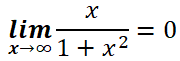
Ejemplo 1. Demostrar que:

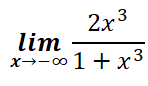
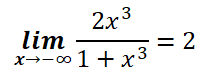
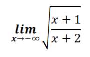
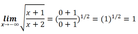
Solución. Por lo general se utiliza un truco común: dividir el numerador y el denominador entre la potencia más alta de x que aparece en el denominador, que en este caso es 2:Ejemplo 2. Encuentre:Solución: 

Por tanto:Ejemplo 3. Encuentre:Solución:Por tanto: 

Escrito por: Profesor Larry Obando – Technical Specialist – Educational Content Writer.

Mentoring Académico / Empresarial / Emprendedores

Copywriting, Content Marketing, Tesis, Monografías, Paper Académicos, White Papers (Español – Inglés)

Escuela de Ingeniería Eléctrica de la Universidad Central de Venezuela, Caracas.

Escuela de Ingeniería Electrónica de la Universidad Simón Bolívar, Valle de Sartenejas.

Escuela de Turismo de la Universidad Simón Bolívar, Núcleo Litoral.

Contact: Caracas, Quito, Guayaquil, Cuenca – Telf. +34633129287

WhatsApp: +34633129287

Control System Analysis, Sin categoría

Dynamik eines Masse-Feder-Dämpfer-Systems

Die Grundelemente eines jeden mechanischen Systems sind die Masse, die Feder und der Stoßdämpfer. Das Studium der Bewegung in mechanischen Systemen entspricht der Analyse dynamischer Systeme. In der Robotik zum Beispiel bezieht sich das Wort Vorwärtsdynamik darauf, was mit Aktuatoren passiert, wenn wir bestimmte Kräfte und Drehmomente auf sie anwenden.

Die Masse, die Feder, der Stoßdämpfer sind elementare Aktuatoren eines mechanischen Systems.

Um den Roboter zu steuern, ist es folglich notwendig, die Art der Bewegung eines Masse-Feder-Dämpfer-Systems sehr gut zu kennen.

Darüber hinaus wird dieses elementare System in vielen Anwendungsbereichen vorgestellt, daher die Wichtigkeit seiner Analyse. Wenn wir in der Robotik über Inverse Dynamic sprechen, sprechen wir darüber, wie man den Roboter auf eine gewünschte Art und Weise bewegt, welche Kräfte und Drehmomente wir auf die Aktoren anwenden müssen, damit sich unser Roboter auf eine bestimmte Art bewegt.

Bevor wir die dynamische Analyse unseres Masse-Feder-Dämpfer-Systems durchführen, müssen wir sein mathematisches Modell erhalten. Dies ist der erste Schritt für jeden, der die Dynamik eines Systems, insbesondere das Verhalten seiner mechanischen Komponenten, genau kennenlernen möchte.

Wir werden unsere Studie mit dem Modell eines Masse-Feder-Systems beginnen.

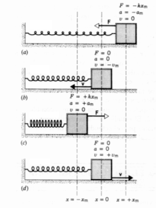
Dies ist aus folgendem Grund praktisch. Alle mechanischen Systeme haben eine Art in ihrer Bewegung, die sie zum Schwingen bringt, etwa wenn ein Gegenstand an einem Faden an der Decke hängt und mit der Hand, die wir drücken. Oder ein Schuh auf einer Plattform mit Federn. Es ist gut zu wissen, welche mathematische Funktion diese Bewegung am besten beschreibt.

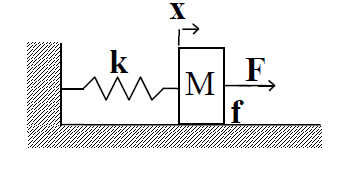
Masse-Feder-System.
Abbildung 5

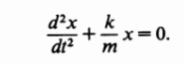
Die Dynamik eines Systems wird in erster Linie durch ein mathematisches Modell dargestellt, das aus Differentialgleichungen besteht. Im Falle des Masse-Feder-Systems ist diese Gleichung wie folgt:

Diese Gleichung ist als Bewegungsgleichung eines einfachen harmonischen Oszillators bekannt. Mal sehen, woher es stammt.

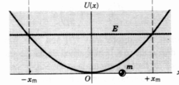
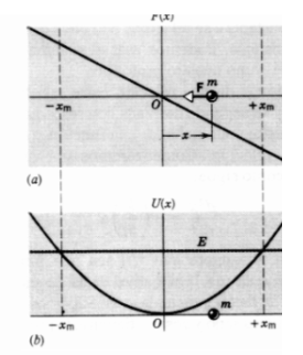
Wenn wir eine Formel erhalten wollen, die die Kraft beschreibt, die eine Feder gegen die Verschiebung ausübt, die sie dehnt oder schrumpft, ist es am besten, die potentielle Energie zu visualisieren, die in die Feder injiziert wird, wenn wir sie dehnen oder schrumpfen. Die folgende Grafik beschreibt, wie sich diese Energie als Funktion der horizontalen Verschiebung verhält:

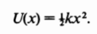
Wenn sich die Masse m der vorhergehenden Figur, die an dem Ende der Feder angebracht ist, wie in Abbildung 5 gezeigt, von dem Federrelaxationspunkt x = 0 weg in die positive oder negative Richtung bewegt, sammelt sich die potentielle Energie U (x) an und steigt in parabolischer Form an und erreicht einen höheren Energiewert, wobei       U(x) = E, Wert, der der maximalen Dehnung oder Kompression der Feder entspricht. Die mathematische Gleichung, die in der Praxis diese Kurvenform am besten beschreibt und eine Konstante k für die physikalische Eigenschaft des Materials enthält, die die Steigung der Kurve erhöht oder verringert, ist die folgende:

Die Kraft ist auf folgende Weise mit der potentiellen Energie verbunden:

Deshalb:

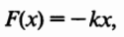
Es ist sinnvoll zu sehen, dass F (x) umgekehrt proportional zur Verschiebung der Masse m ist. Denn es ist klar, dass, wenn wir die Feder dehnen oder schrumpfen, diese Kraft dieser Aktion entgegenwirkt und versucht, die Feder in ihre entspannte oder natürliche Position zurückzubringen. Aus diesem Grund heißt es Restitutionskraft. Die obige Gleichung ist in der Akademie als Hookes Gesetz oder Kraftgesetz für Federn bekannt. Das Folgende ist ein repräsentatives Diagramm dieser Kraft in Bezug auf die Energie, wie sie erwähnt wurde, ohne den Eingriff von Reibungskräften (Dämpfung), weshalb sie als der einfache harmonische Oszillator bekannt ist. Es ist wichtig, die proportionale Beziehung zwischen Verschiebung und Kraft zu betonen, aber mit einer negativen Steigung, und das ist in der Praxis komplexer, nicht linear.

Abbildung 4

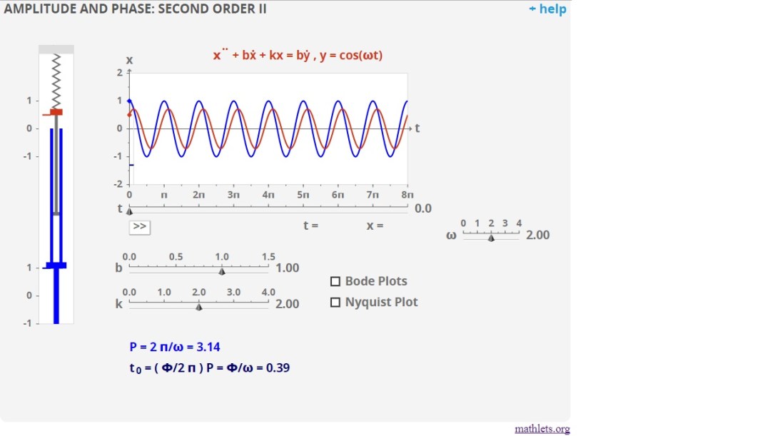
Siehe: AMPLITUDE AND PHASE: SECOND ORDER II (Mathlets)

Sistema MRA

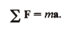
Nach Newtons zweitem Gesetz:

Diese Gleichung sagt uns, dass die vektorielle Summe aller Kräfte, die auf den Körper der Masse m einwirken, gleich dem Produkt des Wertes der Masse aufgrund ihrer Beschleunigung ist, die aufgrund der Kräfte erhalten wird. Mit Newtons zweitem Gesetz erhalten wir die folgende Gleichung:

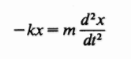
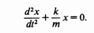
Das ist:

Diese Gleichung repräsentiert die Dynamik eines idealen Masse-Feder-Systems.

System Masse-Feder-Stoßdämpfer

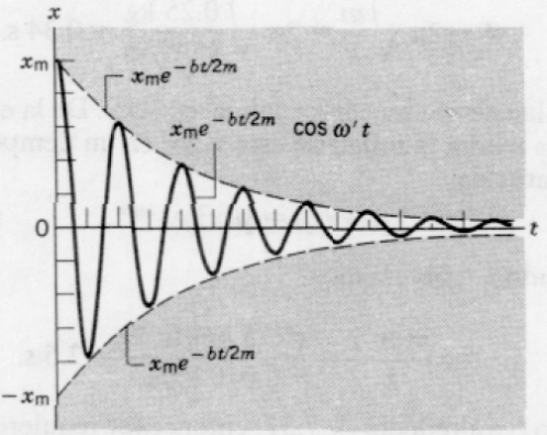
Wenn keine Reibungskraft vorhanden ist, oszilliert der einfache harmonische Oszillator unendlich. In Wirklichkeit nimmt die Amplitude der Oszillation allmählich ab, ein Prozess, der als Dämpfung bekannt ist und im folgenden graphisch beschrieben wird:

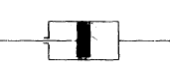
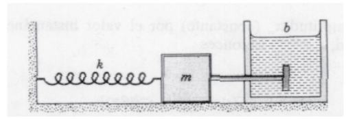
Die Verschiebung einer oszillierenden Bewegung ist gegen die Zeit aufgetragen, und ihre Amplitude wird durch eine sinusförmige Funktion dargestellt, die durch einen abnehmenden Exponentialfaktor gedämpft wird, der in dem Graphen als eine Hüllkurve erscheint. Die Reibungskraft Fv, die auf die amortisierte harmonische Bewegung einwirkt, ist in den meisten Fällen von wissenschaftlichem Interesse proportional zur Geschwindigkeit V. Diese Kraft hat die Form Fv = bV, wobei b eine positive Konstante ist, die unter anderem von den Eigenschaften des Fluids abhängt, das Reibung verursacht. Diese Reibung, auch bekannt als Viskosereibung, wird durch ein Diagramm dargestellt, das aus einem Kolben und einem mit Öl gefüllten Zylinder besteht:

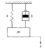
Die gängigste Art, ein Masse-Feder-Dämpfer-System darzustellen, ist eine Reihenschaltung wie folgt:

Abbildung 6

Sowie die folgenden:

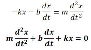
In beiden Fällen wird das gleiche Ergebnis bei Anwendung unserer Analysemethode erhalten. Wenn man Fig. 6 betrachtet, kann man sehen, dass dieselbe Konfiguration wie in Fig. 5 gezeigt ist, jedoch die Wirkung des Stoßdämpfers hinzugefügt wird. Indem wir Newtons zweites Gesetz auf dieses neue System anwenden, erhalten wir die folgende Beziehung:

Diese Gleichung repräsentiert die Dynamik eines Massen-Feder-Schock-Systems.

Das könnte dich interessieren:

  1. Beispiel 1 – System Transfer-Funktion Masse-Feder-Dämpfer
  2. Beispiel 1 – Elektromechanische Systemübertragungsfunktion

Geschrieben von:

Prof. Larry Francis Obando – Technical Specialist – Educational Content Writer 

Escuela de Ingeniería Eléctrica de la Universidad Central de Venezuela, Caracas.

Escuela de Ingeniería Electrónica de la Universidad Simón Bolívar, Valle de Sartenejas.

Escuela de Turismo de la Universidad Simón Bolívar, Núcleo Litoral.

Contact: Caracas, Quito, Guayaquil, Jaén– Telf. +34633129287

WhatsApp: +34633129287

email: dademuchconnection@gmail.com

Sin categoría

Respuesta transitoria de un sistema masa-resorte-amortiguador

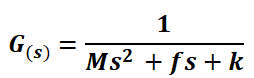
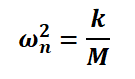
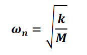
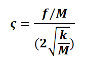
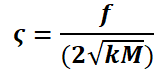
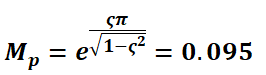
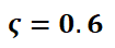
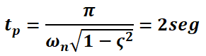
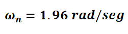
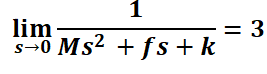
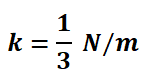
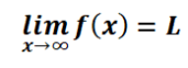
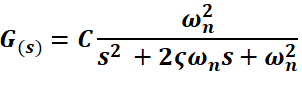
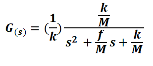
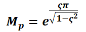
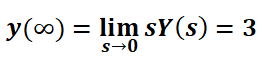
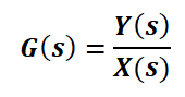
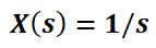
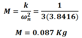
Dada la respuesta del siguiente sistema a una entrada escalón unitario, calcular k, f  y M. null null RESPUESTA La función de transferencia del sistema es: null El sistema de segundo orden prototipo tiene la siguiente forma: null Donde C es una constante. El sistema equivalente queda expresado como: null Donde: null Por tanto:null Por lo que: null null Siendo: null Si suponemos que la curva de la gráfica se corresponde con la función y(t), entonces de la gráfica sabemos que el sobrepaso Mp es: null Por otra parte, en términos del factor de amortiguamiento relativo, Mp es: null null De donde: null Luego, de la gráfica sabemos que: null Por tanto: null Aplicando el teorema del valor final y observando el comportamiento de y(t) cuando t tiende a infinito: null La función de transferencia G(s) nos permite desplegar la expresión para Y(s): null Como la entrada es un escalón unitario: nullPor tanto: nullAsí, volviendo al teorema del valor final: nullDe donde: nullAsí: nullEs decir: null Regresando a la expresión para la frecuencia natural: null null null Por último, null null null


Revisión literaria hecha por:

Prof. Larry Francis Obando – Technical Specialist – Educational Content Writer

Se hacen trabajos, se resuelven ejercicios!!

WhatsApp:  +34633129287  Atención Inmediata!!

Twitter: @dademuch

Copywriting, Content Marketing, Tesis, Monografías, Paper Académicos, White Papers (Español – Inglés)

Escuela de Ingeniería Electrónica de la Universidad Simón Bolívar, USB Valle de Sartenejas.

Escuela de Ingeniería Eléctrica de la Universidad Central de Venezuela, UCV CCs

Escuela de Turismo de la Universidad Simón Bolívar, Núcleo Litoral.

Contacto: España. +34633129287

Caracas, Quito, Guayaquil, Jaén.

WhatsApp:  +34633129287

Twitter: @dademuch

FACEBOOK: DademuchConnection

email: dademuchconnection@gmail.com

Sin categoría

PID – Effect of integrative and derivative control actions

In this section, we shall investigate the effects of integral and derivative control actions on the system performance. Here we shall consider only simple systems so that the effects of integral and derivative control actions on system performance can be clearly seen.

Integral Control Action. In the proportional control of a plant whose transfer function does not possess an integrator 1/s, there is a steady-state error, or offset, in the response to a step input. Such an offset can be eliminated if the integral control action is included in the controller. The main function of the integral action is to ensure that the exit of the process matches the set point in steady state.

In the integral control of a plant, the control signal, the output signal from the controller, at any instant, is the area under the actuating error signal curve up to that instant.

The control signal u(t) can have a nonzero value when the actuating error signal e(t) is zero, as shown in Figure 5-39(a). This is impossible in the case of the proportional controller since a nonzero control signal requires a nonzero actuating error signal.

(A nonzero actuating error signal at steady state means that there is an offset.) Figure

5-39(b) shows the curve e(t) versus t and the corresponding curve u(t) versus t when the

controller is of the proportional type.

Note that integral control action, while removing offset or steady-state error, may lead

to oscillatory response of slowly decreasing amplitude or even increasing amplitude,

both of which are usually undesirable.

Proportional Control of Systems. We shall show that the proportional control of a system without an integrator will result in a steady-state error with a step input. We shall then show that such an error can be eliminated if integral control action is included in the controller.

Consider the system shown in Figure 5-40. Let us obtain the steady-state error in the

unit-step response of this system. Define

Since

the error E(s) is given by

For the unit-step input R(s) = 1/s, we have:

The steady-state error is

Such a system without an integrator in the feedforward path always has a steady-state error in the step response. Such a steady-state error is called an offset. Figure 5-41 shows the unit-step response and the offset.

Integral Control of Systems. Consider the system shown in Figure 5-42. The controller is an integral controller. The closed-loop transfer function of the system is:

Since the system is stable, the steady-state error for the unit-step response can be obtained by applying the final-value theorem, as follows:

Integral control of the system thus eliminates the steady-state error in the response to the step input. This is an important improvement over the proportional control alone, which gives offset.

Derivative Control Action. Derivative control action, when added to a proportional controller, provides a means of obtaining a controller with high sensitivity. An advantage of using derivative control action is that it responds to the rate of change of the actuating error and can produce a significant correction before the magnitude of the actuating error becomes too large. Derivative control thus anticipates the actuating error, initiates an early corrective action, and tends to increase the stability of the system.

Although derivative control does not affect the steady-state error directly, it adds damping to the system and thus permits the use of a larger value of the gain K, which will result in an improvement in the steady-state accuracy. Because derivative control operates on the rate of change of the actuating error and not the actuating error itself, this mode is never used alone. It is always used in combination with proportional or proportional-plus-integral control action.

Proportional Control of Systems with Inertia Load. Before we discuss the effect

of derivative control action on system performance, we shall consider the proportional

control of an inertia load.

Consider the system shown in Figure 5-46(a). The closed-loop transfer function is obtained as:

The characteristic equation is:

Since the roots of the characteristic equation are imaginary, the response to a unit-step input continues to oscillate indefinitely, as shown in Figure 5-46(b). Control systems exhibiting such response characteristics are not desirable. We shall see that the addition of derivative control will stabilize the system.

Proportional-Plus-Derivative Control of a System with Inertia Load. Let us modify the proportional controller to a proportional-plus-derivative controller whose transfer function is Kp(1+Tds). The torque developed by the controller is proportional to Kp(e+Tde’). Derivative control is essentially anticipatory, measures the instantaneous error velocity, and predicts the large overshoot ahead of time and produces an appropriate counteraction before too large an overshoot occurs.

Consider the system shown in Figure 5-47(a).

The closed-loop transfer function is given by:

The characteristic equation is:

Now it has two roots with negative real parts for positive values of J, Kp, and Td. Thus

derivative control introduces a damping effect. A typical response curve c(t) to a unit step

input is shown in Figure 5-47(b). Clearly, the response curve shows a marked improvement over the original response curve shown in Figure 5-46(b).

Proportional-Plus-Derivative Control of Second-Order Systems. A compromise between acceptable transient-response behavior and acceptable steady-state behavior may be achieved by use of proportional-plus-derivative control action. Consider the system shown in Figure 5-48.

The closed-loop transfer function is:

The steady-state error for a unit-ramp input is:

The characteristic equation is:

The effective damping coefficient of this system is thus B + Kd rather than B. Since the

damping ratio of this system is:
it is possible to make both the steady-state error Ess for a ramp input and the maximum

overshoot for a step input small by making B small, Kp large, and Kd large enough so that

is between 0.4 and 0.7.

Sources:

  1. Control PID Avanzado
  2. Modern_Control_Engineering, Ogata 4t p 294

Review by Larry Francis Obando – Technical Specialist – Educational Content Writer

Copywriting, Content Marketing, Tesis, Monografías, Paper Académicos, White Papers (Español – Inglés)

Escuela de Ingeniería Eléctrica de la Universidad Central de Venezuela, CCs.

Escuela de Ingeniería Electrónica de la Universidad Simón Bolívar, Valle de Sartenejas.

Escuela de Turismo de la Universidad Simón Bolívar, Núcleo Litoral.

Contact: Caracas, Quito, Guayaquil, Cuenca. telf – 0998524011

WhatsApp: +593984950376

email: dademuchconnection@gmail.com

Some content on this page was disabled on 3 April, 2020 as a result of a DMCA takedown notice from Pearson Education, Inc.. You can learn more about the DMCA here:

https://wordpress.com/support/copyright-and-the-dmca/

Análisis de sistemas de control, Diagramas de bloques, Sin categoría

Yo le resolveré problemas de Sistemas de Control

Yo le entregaré la solución a cualquier problema típico de la cátedra Sistemas de Control, de las carreras universitarias Ingeniería de Control, Ingeniería Eléctrica, Electrónica, Mecánica, Mecatrónica, Robótica, Matemática y Física Aplicada.

La entrega de la solución en digital incluye además una videoconferencia Skype de una hora, en la cual le explico personalmente a Usted cada paso del método utilizado para llegar a la solución, así como la simulación de la respuesta en Matlab. Tiene por tanto el valor agregado de que le explico cómo utilizar Matlab y su librería Control System Toolbox.

Los temas más solicitados son:

1. Análisis en el tiempo del sistema masa-resorte-amortiguador, simulación en Matlab.

2. Diagrama de bloques y Función de Transferencia de Sistemas Electromecánicos (que incluyen motores, amplificadores, niveles de líquido, servomotores ), simulación en Matlab

3. Análisis en Variables de Estado, Respuesta en Frecuencia, Lugar Geométrico de las raíces

4. Respuesta del sistema a las acciones de control Integral y Derivativa, Control PID.

5. Diseño de sistemas de control, compensación de atraso-adelanto

6. Todo tipo de solución simulada en Matlab. Gráficas, asesoría en el uso de Matlab Control System Toolbox, Simulink. A continuación una descripción de costos según paquete contratado

Paquetes


Básico 15$


Estándar 20$


Premium 25$

Análisis de Sistemas Masa-Resorte-Amortiguador. Incluye:


Ecuaciones de dinámica.

Análisis en el tiempo. Transformada de Laplace.

Función de Transferencia.

Simulación en Matlab

Videoconferencia 1hr.

Diagrama de bloques y Función de Transferencia de Sistemas de Control. Todo del paquete básico más:

Diagrama de bloques y Función de Transferencia de sistemas de control electromecánicos (que involucran motores, sensores, amplificadores, etc), hidráulicos (niveles y presión de líquidos), de temperatura, etc..


Análisis y Diseño de Sistemas de Control. Incluye:


Análisis y diseño de sistemas de control en Variables de Estado, Respuesta en Frecuencia, Lugar Geométrico de las Raíces, Control PID, Compensación.

Simulación en Matlab

Videoconferencia 1hr.

Tiempo de entrega:

  1. 2 días
  2. 1 día (+5$)
  3. 2 horas (+15$)
Tiempo de entrega:

  1. 2 días
  2. 1 día (+5$)
  3. 2 horas (+15$)
Tiempo de entrega:

  1. 2 días
  2. 1 día (+5$)
  3. 4 horas (+15$)

Observación: para estudiantes de ingeniería en Venezuela el servicio se negocia en términos de cooperación institucional, no en términos monetarios.

Prof. Larry Francis Obando – Technical Specialist

Escuela de Ingeniería Eléctrica de la Universidad Central de Venezuela, CCs.

Escuela de Ingeniería Electrónica de la Universidad Simón Bolívar, Valle de Sartenejas.

Escuela de Turismo de la Universidad Simón Bolívar, Núcleo Litoral.

Le ruego se comunique conmigo a través de las siguientes alternativas:

  1. WhatsApp: +593981478463
  2. email: dademuchconnection@gmail.com
  3. Teléfono: 00593 – 998524011 (desde el extranjero) / 0998524011 (en Ecuador).

I write the solution to typical problems of the Control Systems at Schools of Electrical Engineering, Electronics, Mechanics, Mechatronics, Robotics, Applied Mathematics, Applied Physics.

The delivery of the response includes a video-conference of one hour or more depending on the package contracted, to explain the solution. The consultant provides the entire bibliographic resources.

1. The analysis in time of the mass-spring-damper system, simulation in Matlab.

2. Block Diagram and Transfer Function of Electromechanical Systems (including motors, amplifiers, liquid levels, servomotors), simulation in Matlab

3. Analysis of State Variables, Frequency Response, Geometrical Place of Roots

4. System response to Integral and Derivative control actions, PID Control.

5. Design of control systems, delay-advance compensation

6. All types of simulated solution in Matlab. Graphics, advice on the use of Matlab Control System Toolbox, Simulink.

Please contact me through the follows:

  1. WhatsApp: +593984950376
  2. email: dademuchconnection@gmail.com
  3. Teléfono: 00593 – 998524011 (desde el extranjero) / 0998524011 (en Ecuador).

I am a proficient English writer and speaker.

Compare Packages


Basic 15$


Standard 20$


Premium 25$

Analysis of Mass-Spring-Damper Systems. It includes:


Dynamics equations.

Analysis in time.

Laplace Transform.

Transfer function.

Simulation in Matlab

Videoconference 1hr.

Block diagram and Control System Transfer Function. All of the basic package plus:

Block diagram and the transfer function of electromechanical control systems (involving motors, sensors, amplifiers, etc.), hydraulic (liquid levels and pressure), temperature, etc.


Analysis and Design of Control Systems. It includes:


Analysis and design of control systems in State Variables, Frequency Response, Root Geometrical Place, PID Control, Compensation.

Simulation in Matlab

Videoconference 1hr.

Delivery Time:

  1. 2 days
  2. 1 day (+5$)
  3. 2 hours (+15$)
Delivery Time:

  1. 2 days
  2. 1 day (+5$)
  3. 2 hours (+15$)
Delivery Time:

  1. 2 days
  2. 1 day (+5$)
  3. 2 hours (+15$)
Circuit Analysis, Ecuaciones Diferenciales, Electrical Engineer, Elementos Básicos, Literature Review, Señales y Sistemas, Sin categoría

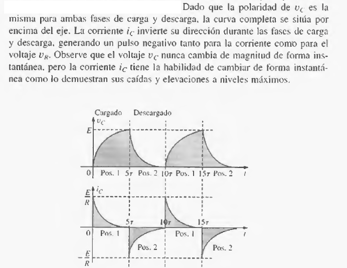
EL CAPACITOR. Relación corriente-voltaje.

Formalmente, la Capacitancia es la razón entre la carga de una placa del capacitor y la diferencia de tensión entre las dos placas:

null

Relación corriente-voltaje del capacitor

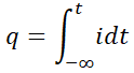
Para obtener la relación de corriente-tensión del capacitor, primero es necesario estudiar la relación entre la carga q y la corriente i. Dicha relación viene dada por la ecuación:

null

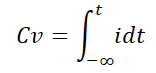
Para encontrar la carga q de las placas en el tiempo t se integra sobre todo el tiempo anterior:

null

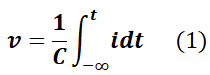
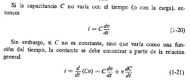
Utilizando el hecho de que q=Cv, obtenemos la relación corriente-tensión del capacitor (suponiendo un capacitor lineal, es decir, que no depende del valor de la tensión v en el tiempo):

null

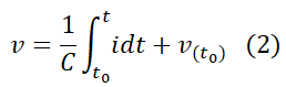
null

O sea:

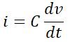
null

Otra forma de presentar este resultado es mediante la fórmula:

null

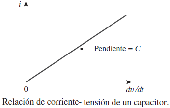
Utilizando esta última ecuación, podemos graficar la relación corriente-voltaje del capacitor de la manera siguiente:

null

Recomiendo leer la siguiente guía: Capacitores e Inductores – Circuitos y asociaciones

Preliminares

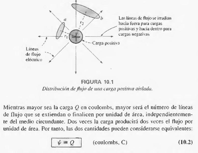
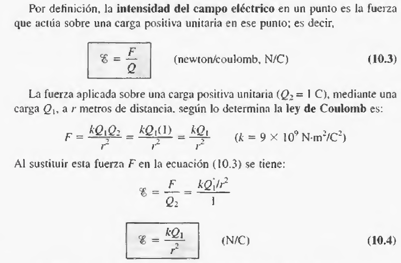
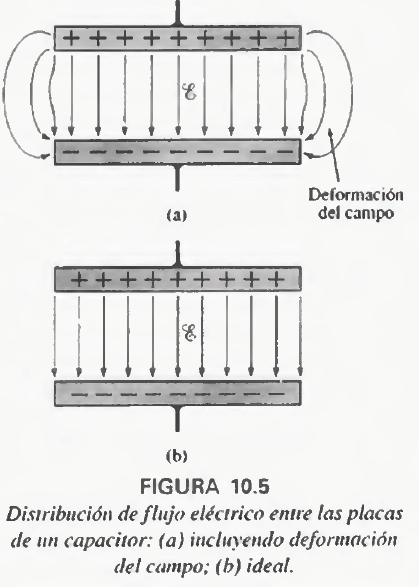
Por tanto se concluye que la intensidad del campo eléctrico en cualquier punto a una distancia r de una carga puntual de Q coulombs, será directamente proporcional a la magnitud de la carga e inversamente proporcional al cuadrado de la distancia a la carga.

Capacitancia

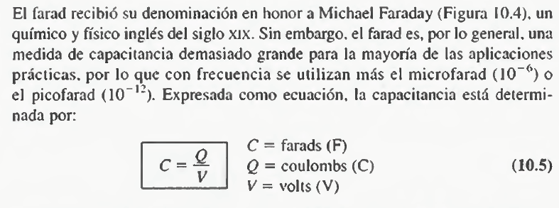
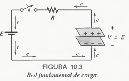
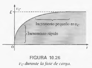
Al instante en que el interruptor se cierra, se extraen los electrones de la placa superior y se depositan sobre la placa inferior debido a la batería, dando por resultado una carga neta positiva sobre la placa superior del capacitor y una carga negativa sobre la placa inferior…Cuando el voltaje en el capacitor es igual al de la batería, cesa la transferencia de electrones y la placa tendrá una carga neta Q=CV=CE

En este punto el capacitor asumirá las características de un circuito abierto: una caída de voltaje en las placas sin flujo de carga entre las placas.

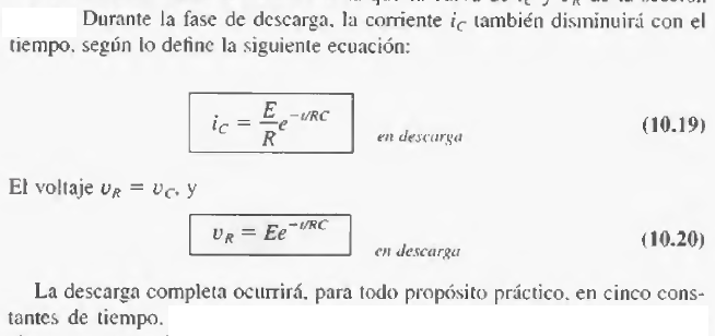
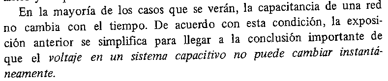
El voltaje en un capacitor no puede cambiar de forma instantánea.

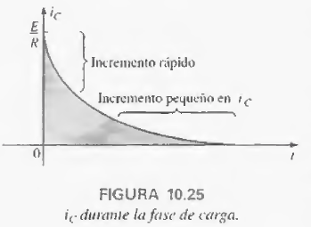
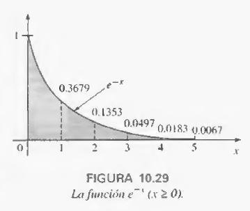
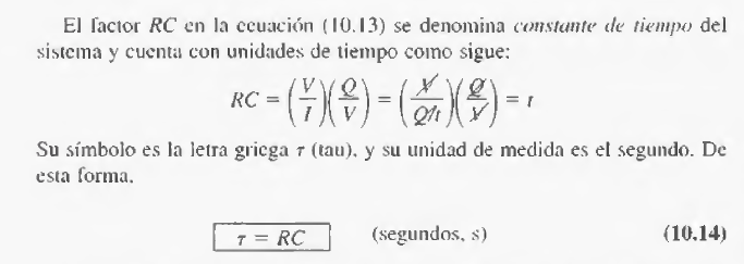
De hecho, la capacitancia en una red es también una medida de cuanto se opondrá ésta a un cambio en el voltaje de la red. Mientras mayor sea la capacitancia, mayor será la constante de tiempo y mayor el tiempo que le tomará cargar hasta su valor final

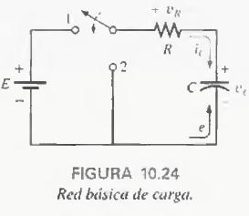
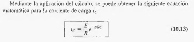
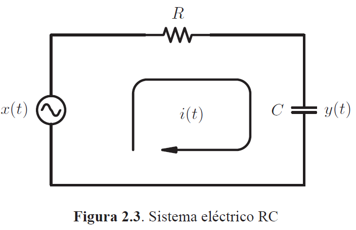
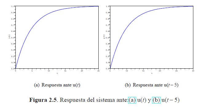
Ejemplo 2.2 (Fuente:3) La Figura 2.3 muestra un sistema compuesto por una resistencia y un capacitor, y cuyos valores son representados respectivamente por R y C. Además, la figura muestra que el sistema eléctrico es excitado por una señal x(t) = u(t) y su respuesta es medida a través de la tensión sobre el capacitor, donde u(t) representa la función escalón unitario:

El modelo matemático asociado al sistema representado por la Figura 2.3 puede obtenerse empleando elementales ecuación de redes eléctricas:

Entonces, al comparar el modelo matemático definido por la Ecuación (2.12) con el modelo obtenido, se tiene que el coeficiente a0 y la señal de excitación son:

,

Al aplicar la solución expresada por medio de la Ecuación (2.21), se puede afirmar que:

Al operar la Ecuación (2.26) se tiene que la respuesta del sistema es dada por:

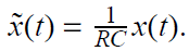
Note que:

por cuanto el elemento de memoria representado por el capacitor no permite cambios bruscos y por tal motivo y(0-) = y(0) = y(0+). Además, para buscar una respuesta a la pregunta debe tomarse en cuenta que la excitación tiene un valor de cero y ella ha permanecido en cero desde mucho tiempo atrás, es decir, desde menos infinito, obviamente y(0) = 0.

Recomiendo leer la siguiente guía: Capacitores e Inductores – Circuitos y asociaciones

Fuentes:

  1. Introduccion-al-analisis-de-circuitos-robert-l-boylestad,
    1. El Parámetro Capacitancia p 20
  2. Análisis de Redes – Van Valkenburg,
    1. El Parámetro Capacitancia p 20
  3. Análisis de Sistemas Lineales – Prof. Ebert Brea
    1. Análisis de Sistemas en el Dominio Continuo pp 29 –
  4. Fundamentos_de_circuitos_electricos_5ta

SIGUIENTE:

Escrito por Prof. Larry Francis Obando – Technical Specialist – Educational Content Writer – Twitter: @dademuch

Se hacen ejercicios, problemas, trabajos, clases online…Respuesta inmediata !!! a través de: WhatsApp: +34 633129287

Mentoring Académico / Emprendedores / Empresarial

Copywriting, Content Marketing, Tesis, Monografías, Paper Académicos, White Papers (Español – Inglés)

Escuela de Ingeniería Electrónica de la Universidad Simón Bolívar, USB Valle de Sartenejas.

Escuela de Ingeniería Eléctrica de la Universidad Central de Venezuela, UCV CCs

Escuela de Turismo de la Universidad Simón Bolívar, Núcleo Litoral.

Contacto: Jaén – España: Tlf. 633129287

Caracas, Valladolid, Quito, Guayaquil, Jaén, Ordizia, Zaragoza.

WhatsApp: +34 633129287

Twitter: @dademuch

FACEBOOK: DademuchConnection

email: dademuchconnection@gmail.com

Sin categoría

Ocho (8) hábitos mentales esenciales para el éxito en la elaboración de material escrito.

El «Council of writing program administrators», el «National council of teahcers of English», y el «National writing project», han identificado estos 8 hábitos como esenciales para el éxito como escritor:

  • Curiosity: the desire o know more about the world;
  • Opennes: the willingness to consider new ways of being and thinking in the world;
  • Engagement: a sense of invesment and involvement in learning;
  •  Creativity: the ability to use novel approaches for generating, investigating, and representing ideas;
  • Persistence: the ability to sustain interest in and attention to short – and long – term projects;
  • Responsability: the ability to take ownership of one´s action and understand the consequences of those actions for oneself and others;
  • Flexibility: the ability to adapt to situations, expectations, or demands;
  • Metacognition: the ability to reflect on one´s own thinking as well as the individual and cultural processes used to structure knowledge.

El documento siguiente provee de una explicación completa sobre cada hábito:

Framework-for-success-postsecondary-writing