“A building created to give its users the most efficient environment; at the same time, the building utilizes and manages resources efficiently and minimizes the life costs of hardware and facilities”;
The approaches to defining an IB can be grouped into three categories as listed below:
Performance- based definitions;
Services- based definitions;
System- based definitions.
Performance-based definition
Performance- based IB definitions emphasize building performance and the demands of users rather than the technologies or systems provided. According to this category of definition, owners and developers of buildings need to understand correctly what kind of buildings they want and also how to satisfy continuously the increasing demands of users. Energy and environmental performances of buildings are certainly among the important issues of an IB. An intelligent building should also adapt itself quickly in response to internal and external conditions, and to meet the changing demands of users.
A typical performance- based IB definition may be that of the European Intelligent Building Group (EIBG) located in the United Kingdom. It defines an IB as:
“a building created to give its users the most efficient environment; at the same time, the building utilizes and manages resources efficiently and minimizes the life costs of hardware and facilities”;
Another example of a performance- based definition is that given by the Intelligent Building Institute (IBI) in the United States, which states that:
“an IB provides a highly efficient, comfortable and convenient environment by satisfying four fundamental demands: structure, system, service and management, and optimizing their interrelationship”.
Service-based definition
Services- based definitions describe IBs from the viewpoint of services and/or quality of services provided by buildings. The Japanese Intelligent Building Institute (JIBI) provides an example of a services- based definition:
“an IB is a building with the service functions of communication, office automation and building automation, and is convenient for intelligent activities”.
The key issues of IBs in Japan focus on the following four services aspects:
Serving as a locus for receiving and transmitting information and supporting efficient management;
Ensuring satisfaction and convenience of persons working inside;
Rationalization of building management to provide more attractive administrative services at lower cost;
Fast, flexible and economical responses to the changing sociological environment, diverse and complex working demands and active business strategies.
System-based definition
System- based IB definitions describe IBs by directly addressing the technologies and technology systems that IBs should include. A typical system- based IB definition is the one suggested in the Chinese IB Design Standard (GB/T50314–2000), which states that:
“IBs provide building automation, office automation and communication network systems, and an optimal composition integrates the structure, system, service and management, providing the building with high efficiency, comfort, convenience and safety to users”.
A more straightforward system- based IB definition has been used by some professionals and developers in practice. It labels the IBs as ‘3A’, which represents building automation (BA), communication automation (CA) and office automation (OA).
Source: Intelligent Buildings and Building Automation, 2010 Edition
Literature review by:
Prof. Larry Francis Obando – Technical Specialist – Educational Content Writer
Mentoring Académico / Emprendedores / Empresarial
Copywriting, Content Marketing, Tesis, Monografías, Paper Académicos, White Papers (Español – Inglés)
Escuela de Ingeniería Eléctrica de la Universidad Central de Venezuela, UCV CCs
Escuela de Ingeniería Electrónica de la Universidad Simón Bolívar, USB Valle de Sartenejas.
Escuela de Turismo de la Universidad Simón Bolívar, Núcleo Litoral.
Por lo general, describimos la frecuencia como el número de días por semana. En atletas de élite, la frecuencia se refiere también al número de semanas por mes o meses por año, porque el entrenamiento apunta hacia una competencia. El entrenamiento de los atletas de alto rendimiento en la temporada temprana es diferente a su entrenamiento en la última parte de la temporada, también conocidos como micro y macro ciclos.
Enfocando el tema en días por semana, ¿por qué no entrenamos siete días a la semana?
La clave, la señal para la adaptación, es el daño muscular. Si es daño, entonces tenemos que darle tiempo al músculo para recuperarse. De lo contrario, creamos un poco de daño, no se recupera, la próxima vez que hagamos ejercicio, crea un poco más de daño, y luego un poco más. Y terminamos en un círculo vicioso.
Así que queremos hacer ejercicio, crear un poco de daño, y crear así una señal para fortalecernos. Una vez que nos recuperamos, nos volvemos más fuertes. Los músculos se vuelven más fuertes, y cuando hacemos ejercicio nuevamente, obtenemos un ciclo positivo de adaptación.
La falta de una recuperación adecuada es probablemente la hipótesis principal de lo que muchos llaman lesión por uso excesivo. ¿Pero es realmente una lesión por uso excesivo?
Steve Stovitz en la Universidad de Minnesota, lo llama lesión por uso insuficiente. Y su criterio es muy simple. Ha habido estudios en los que llevan a personas, y piensan en el entrenamiento militar y básico. Todos pasan por el mismo uso exacto, los mismos ejercicios de formación básicos. Algunas personas no se lesionan porque están en forma . Las personas que no están en forma, que no han usado su cuerpo durante cierto tiempo, son las que se lesionan. Así que han subutilizado el cuerpo. El problema es que se somete al cuerpo a una carga excesiva en comparación con lo que el cuerpo acostumbra a tolerar regularmente.
Entonces, ¿cuánta recuperación necesitamos? Bueno, eso depende de cuánto daño vas a causar al músculo.
Cuando corres maratones, el daño es diferente a cuando estás levantando pesas. Si estás levantando pesos pesados, vas a ocasionar un poco más de daño. Por tanto, necesitarás un poco más de tiempo para que el músculo se regenere.
Ahora, cuanto más alta es la intensidad, más larga es la recuperación.
La mayoría de los libros hablarán sobre cómo debe entrenarse de tres a cuatro veces por semana para obtener algún tipo de beneficio. Algunos grupos en particular dicen que solo tienes que entrenar una o dos veces por semana.
Si la intensidad es moderada, en términos generales, hablamos de dos veces por semana para mantener, de tres a cuatro veces por semana para beneficiarnos. Si entrenas intensidad moderada todos los días y tu cuerpo no está preparado para ello, entrarás en el ciclo negativo. Pero si estás entrenando poco, como caminar o hacer ejercicios ligeros, entonces no hay problema. Puedes entrenar todos los días.
Es todo el mismo principio. Solo tienes que darle tiempo al músculo para que se recupere.
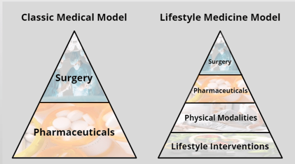
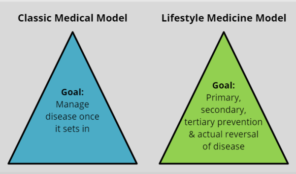
Lifestyle Medicine es la ciencia y la aplicación de estilos de vida saludables que intervienen para la prevención y el tratamiento de enfermedades relacionadas con el estilo de vida, como enfermedades cardíacas, diabetes, derrames cerebrales, obesidad, algunas afecciones neurológicas y algunos tipos de cáncer. Es la especialidad basada en la evidencia que une la ciencia de la actividad física, la nutrición, el manejo del estrés y la resiliencia, la higiene del sueño y otros hábitos saludables para los individuos a través de la práctica clínica en cuidado de la salud.
El mejor secreto de la medicina es el poder de la nutrición, cuando el cuerpo se cura a sí mismo. Esta es la mejor inversión que una persona puede hacer. (The Best Kept Secret in Medicine).
La intervención en el estilo de vida (Lifestyle intervention) es un elemento clave de la prevención y el control de la hipertensión, la insuficiencia cardíaca, las enfermedades cardiovasculares, los accidentes cerebrovasculares, el cáncer, la diabetes y la muerte por todas las causas. Esto porque reduce la presión arterial, la glucosa, el colesterol e influye en las causas fundamentales y los mecanismos biológicos que conducen a la enfermedad. Por ejemplo, en un estudio sobre la salud de las enfermeras se encontró que el riesgo de enfermedad coronaria 15 y diabetes mellitus tipo 216 se redujo 5 y 10 veces, respectivamente, entre los que participaron en 5 comportamientos saludables modificables.
Cuadro comparativo:
Los resultados del siguiente estudio nacional realizado en el año 2000: Healthy_lifestyle_characteristics_2000, muestran que solo el 3.0% de los adultos de EE. UU. siguieron una combinación de 4 características de estilo de vida modificables: no fumar, peso saludable, consumo adecuado de frutas y verduras, y actividad física regular. Ningún subgrupo se involucró en los 4 estilos de vida saludables en ningún grado importante; el predominio más alto es solo del 5.7%. Estos resultados ilustran el extraordinariamente bajo predominio de estilos de vida saludables en la población adulta de EE. UU.
En la Tabla 2 se muestran las estimaciones de predominio ajustadas por edad del indicador de estilo de vida saludable (es decir, la participación en las 4 Healthy Lifestyle Characteristics or HLCs for short) según las 6 variables demográficas y relacionadas con la salud.
El predominio general fue de solo el 3.0% y las diferencias absolutas entre los subgrupos fueron pequeñas, con un rango desde el 0.8% (en personas con educación inferior a la secundaria) hasta solo el 5.7% (en personas con excelente salud):
Los objetivos de este estudio fueron informar sobre el predominio de las características del estilo de vida saludable (HLCs) y generar un indicador único de un estilo de vida saludable.
Definimos los siguientes 4HLCs: no fumador; peso saludable (índice de masa corporal [calculado como peso en kilogramos dividido por el cuadrado de la altura en metros] de 18.5-25.0); consumir 5 o más frutas y verduras por día; y actividad física regular (30 minutos por 5 veces por semana).
Las 4 HLCs se sumaron para crear un índice de estilo de vida saludable (rango, 0-4), y el patrón de seguimiento de las 4 HLCs se definió como un único indicador de estilo de vida saludable.
Al utilizar datos de más de 153 000 adultos, el predominio (intervalo de confianza del 95%) de las HLCs individuales fue la siguiente: no fumadores, 76.0% (75.6% -76.4%); peso saludable, 40.1% (39.7% -40.5%); 5 frutas y verduras por día, 23.3% (22.9% -23.7%); y actividad física regular, 22.2% (21.8% -22.6%). El predominio general del indicador de estilo de vida saludable (es decir, que tiene las 4 HLCs) fue de solo el 3,0% (intervalo de confianza del 95%, 2,8% -3,2%), con poca variación entre los subgrupos (rango, 0,8% -5,7%).
Conclusión: estos datos ilustran que muy pocos adultos en los Estados Unidos llevan a cabo un estilo de vida saludable, definido como una combinación de 4 HLCs, y que ningún subgrupo siguió esta combinación a un nivel remotamente compatible con las recomendaciones clínicas o de salud pública.
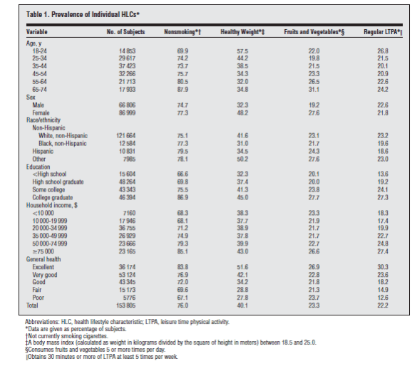
Las estimaciones de predominio de cada HLCs según las 6 variables demográficas y relacionadas con la salud se muestran en la Tabla 1:
El setenta y seis por ciento (95% CI, 75.6% -76.4%) de los adultos de EE. UU. no fuma cigarrillos actualmente. Esta tendencia se mostró fuertemente positiva al aumentar la edad, la educación, los ingresos familiares y el estado de salud. Solo el 40,1% (95% CI, 39,7-40,5%) de los adultos tenía peso saludable, que mostró una fuerte tendencia inversa con la edad y tendencias positivas con la educación y el estado de salud. El peso saludable fue más común en las mujeres y entre los blancos. Solo el 23.3% (95% CI, 22.9% -23.7%) de las personas consumió frutas y verduras 5 o más veces por día, mientras que el LTPA (Leisure Time Physical Activity) regular se realizó en solo 22.2% (95% CI, 21.8% -22.6%).
Comentarios:
Los resultados generados a partir de esta base de datos representativa a nivel nacional indican que solo el 3.0% de los adultos de EE. UU. siguieron una combinación de 4 características de estilo de vida modificables: no fumar, peso saludable, consumo adecuado de frutas y verduras, y actividad física regular. Ningún subgrupo se involucró en los 4 estilos de vida saludables en ningún grado importante; el predominio más alto fue de solo el 5.7%. Estos resultados ilustran el extraordinariamente bajo predominio de los estilos de vida saludables en la población adulta de EE. UU. Revisión Bibliográfica:
Date: February 2019, Location: Caracas, Quito, Guayaquil.
Lifestyle Medicine is the science and application of healthy lifestyles as interventions for the prevention and treatment of lifestyle-related diseases such as heart disease, diabetes, stroke, obesity, some neurological conditions and some cancers. It is the evidence-based specialty bridging the science of physical activity, nutrition, stress management and resilience; sleep hygiene and other healthy habits to individuals through clinical practice in healthcare.
The best keep secret in medicine is the power of nutrition, when the body heals himself. This is the best investment you can make (The Best Kept Secret in Medicine).
Lifestyle intervention is a key element of prevention and control of hypertension, heart failure, cardiovascular disease, stroke, cancer, diabetes, and death from all causes. This because it reduces blood pressure, glucose, cholesterol, and influence the fundamental causes and biological mechanisms leading to disease. For example, the Nurses’ Health Study found that the risk of coronary heart disease15 and type 2 diabetes mellitus16 was reduced 5- and 10-fold, respectively, among those who engaged in 5 modifiable healthy behaviors.
Comparative chart:
The results from this nationally representative database 2000 Study: Healthy_lifestyle_characteristics_2000, show that just 3.0% of US adults followed a combination of 4 modifiable lifestyle characteristics— nonsmoking, healthy weight, adequate fruit and vegetable consumption, and regular physical activity. No subgroup engaged in all 4 healthy lifestyles to any important degree— the highest prevalence being only 5.7%. These results illustrate the extraordinarily low prevalence of healthy lifestyles in the US adult population.
The age-adjusted prevalence estimates of the healthy lifestyle indicator (ie, engaging in all 4 HLCs) by the 6 demographic and health-related variables are shown in Table 2.
The overall prevalence was only 3.0%, and the absolute differences across subgroups were small, ranging from 0.8% (in persons with less than high school education) to only 5.7% (in persons in excellent health):
The objectives of this study were to report on the prevalence of healthy lifestyle characteristics (HLCs) and to generate a single indicator of a healthy lifestyle.
We defined the following 4 HLCs: nonsmoking, healthy weight (body mass index [calculated as weight in kilograms divided by the square of height in meters] of 18.5-25.0), consuming 5 or more fruits and vegetables per day, and regular physical activity (30 minutes for5 times per week).
The 4 HLCs were summed to create a healthy lifestyle index (range, 0-4), and the pattern of following all 4 HLCs was defined as a single healthy lifestyle indicator.
By using data from more than 153 000 adults, the prevalence (95% confidence interval) of the individual HLCs was as follows: nonsmoking, 76.0% (75.6%-76.4%); healthy weight, 40.1% (39.7%-40.5%); 5 fruits and vegetables per day, 23.3% (22.9%-23.7%); and regular physical activity, 22.2% (21.8%-22.6%). The overall prevalence of the healthy lifestyle indicator (ie, having all 4 HLCs) was only 3.0% (95% confidence interval, 2.8%-3.2%), with little variation among subgroups (range, 0.8%-5.7%).
Conclusion: These data illustrate that a healthy lifestyle— defined as a combination of 4 HLCs—was undertaken by very few adults in the United States, and that no subgroup followed this combination to a level remotely consistent with clinical or public health recommendations.
The prevalence estimates of each HLC by the 6 demographic and health-related variables are shown in Table1:
Seventy-six percent (95% CI, 75.6%-76.4%) of US adults did not currently smoke cigarettes. Nonsmoking showed strong positive trends with increasing age, education, household income, and health status. Only 40.1% (95% CI, 39.7-40.5%) of adults had healthy weight, which showed a strong inverse trend with age and positive trends with education and health status. Healthy weight was more common in women and among whites. Only 23.3% (95% CI, 22.9%-23.7%) of persons consumed fruits and vegetables 5 or more times per day, while regular LTPA was undertaken by only 22.2% (95% CI, 21.8%-22.6%).
Comments:
The results generated from this nationally representative database indicate that just 3.0% of US adults followed a combination of 4 modifiable lifestyle characteristics— nonsmoking, healthy weight, adequate fruit and vegetable consumption, and regular physical activity. No subgroup engaged in all 4 healthy lifestyles to any important degree— the highest prevalence being only 5.7%. These results illustrate the extraordinarily low prevalence of healthy lifestyles in the US adult population.
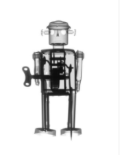
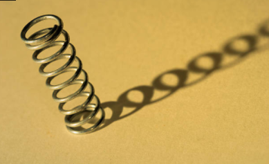
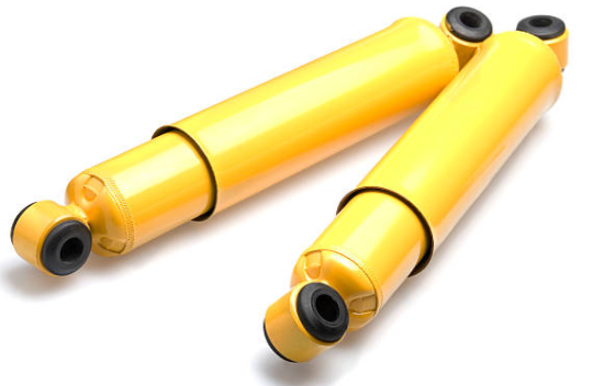
The basic elements of any mechanical system are the mass, the spring and the shock absorber, or damper. The study of movement in mechanical systems corresponds to the analysis of dynamic systems. In Robotics, for example, the word Forward Dynamic refers to what happens to actuators when we apply certain forces and torques to them.
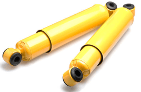
The mass, the spring and the damper are basic actuators of the mechanical systems.
Consequently, to control the robot it is necessary to know very well the nature of the movement of a mass-spring-damper system.
In addition, this elementary system is presented in many fields of application, hence the importance of its analysis. Again, in robotics, when we talk about Inverse Dynamic, we talk about how to make the robot move in a desired way, what forces and torques we must apply on the actuators so that our robot moves in a particular way.
I recommend the book «Mass-spring-damper system, 73 Exercises Resolved and Explained» I have written it after grouping, ordering and solving the most frequent exercises in the books that are used in the university classes of Systems Engineering Control, Mechanics, Electronics, Mechatronics and Electromechanics, among others.
If you need to acquire the problem solving skills, this is an excellent option to train and be effective when presenting exams, or have a solid base to start a career on this field. Take a look at the Index at the end of this article.
Before performing the Dynamic Analysis of our mass-spring-damper system, we must obtain its mathematical model. This is the first step to be executed by anyone who wants to know in depth the dynamics of a system, especially the behavior of its mechanical components.
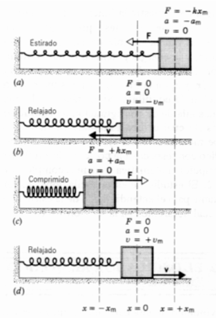
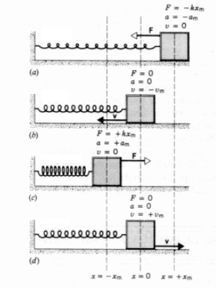
We will begin our study with the model of a mass-spring system.
This is convenient for the following reason. All the mechanical systems have a nature in their movement that drives them to oscillate, as when an object hangs from a thread on the ceiling and with the hand we push it. Or a shoe on a platform with springs. It is good to know which mathematical function best describes that movement.
But it turns out that the oscillations of our examples are not endless. There is a friction force that dampens movement. In the case of the object that hangs from a thread is the air, a fluid. So after studying the case of an ideal mass-spring system, without damping, we will consider this friction force and add to the function already found a new factor that describes the decay of the movement.
Mass-Spring System.
Figure 5
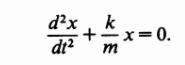
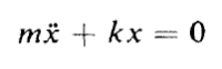
The dynamics of a system is represented in the first place by a mathematical model composed of differential equations. In the case of the mass-spring system, said equation is as follows:
This equation is known as the Equation of Motion of a Simple Harmonic Oscillator. Let’s see where it is derived from.
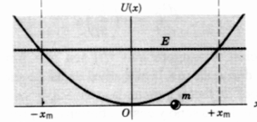
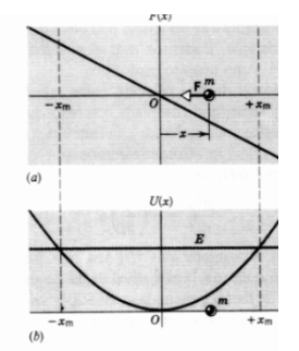
If our intention is to obtain a formula that describes the force exerted by a spring against the displacement that stretches or shrinks it, the best way is to visualize the potential energy that is injected into the spring when we try to stretch or shrink it. The following graph describes how this energy behaves as a function of horizontal displacement:
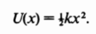
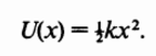
As the mass mof the previous figure, attached to the end of the spring as shown in Figure 5, moves away from the spring relaxation point x = 0 in the positive or negative direction, the potential energy U (x) accumulates and increases in parabolic form, reaching a higher value of energy where U (x) = E, value that corresponds to the maximum elongation or compression of the spring. The mathematical equation that in practice best describes this form of curve, incorporating a constant k for the physical property of the material that increases or decreases the inclination of said curve, is as follows:
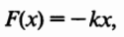
The force is related to the potential energy as follows:
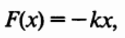
Therefore:
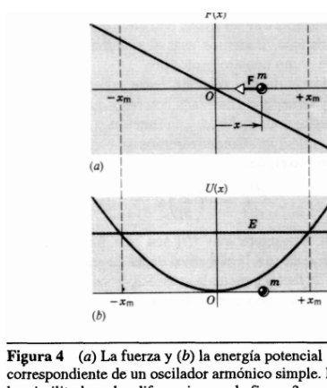
It makes sense to see that F (x) is inversely proportional to the displacement of mass m. Because it is clear that if we stretch the spring, or shrink it, this force opposes this action, trying to return the spring to its relaxed or natural position. For that reason it is called restitution force. The above equation is known in the academy as Hooke’s Law, or law of force for springs. The following is a representative graph of said force, in relation to the energy as it has been mentioned, without the intervention of friction forces (damping), for which reason it is known as the Simple Harmonic Oscillator. It is important to emphasize the proportional relationship between displacement and force, but with a negative slope, and that, in practice, it is more complex, not linear.
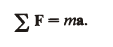
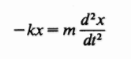
This equation tells us that the vectorial sum of all the forces that act on the body of mass m, is equal to the product of the value of said mass due to its acceleration acquired due to said forces. Considering that in our spring-mass system, ΣF = -kx, and remembering that acceleration is the second derivative of displacement, applying Newton’s Second Law we obtain the following equation:
Fixing things a bit, we get the equation we wanted to get from the beginning:
This equation represents the Dynamics of an ideal Mass-Spring System.
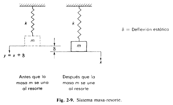
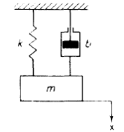
Apart from Figure 5, another common way to represent this system is through the following configuration:
:
In this case we must consider the influence of weight on the sum of forces that act on the body of mass m. The weight P is determined by the equation P = m.g, where g is the value of the acceleration of the body in free fall.
If the mass is pulled down and then released, the restoring force of the spring acts, causing an acceleration ÿ in the body of mass m. We obtain the following relationship by applying Newton:
If we implicitly consider the static deflection, that is, if we perform the measurements from the equilibrium level of the mass hanging from the spring without moving, then we can ignore and discard the influence of the weight P in the equation. If we do y = x, we get this equation again:
Mass-spring-damper System
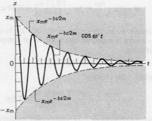
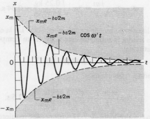
If there is no friction force, the simple harmonic oscillator oscillates infinitely. In reality, the amplitude of the oscillation gradually decreases, a process known as damping, described graphically as follows:
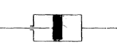
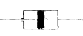
The displacement of an oscillatory movement is plotted against time, and its amplitude is represented by a sinusoidal function damped by a decreasing exponential factor that in the graph manifests itself as an envelope. The friction force Fv acting on the Amortized Harmonic Movement is proportional to the velocity Vin most cases of scientific interest. This force has the form Fv = bV, where b is a positive constant that depends on the characteristics of the fluid that causes friction. This friction, also known as Viscose Friction, is represented by a diagram consisting of a piston and a cylinder filled with oil:
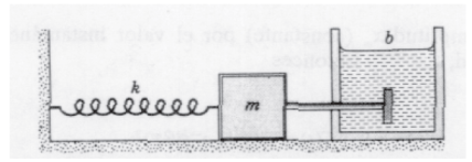
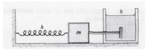
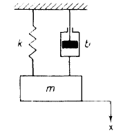
The most popular way to represent a mass-spring-damper system is through a series connection like the following:
Figura 6
As well as the following:
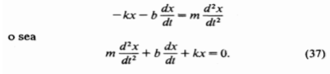
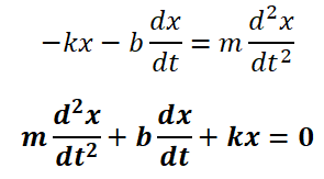
In both cases, the same result is obtained when applying our analysis method. Considering Figure 6, we can observe that it is the same configuration shown in Figure 5, but adding the effect of the shock absorber. Applying Newton’s second Law to this new system, we obtain the following relationship:
This equation represents the Dynamics of a Mass-Spring-Damper System.
Laplace Transform of a Mass-Spring-Damper System
A solution for equation (37) is presented below:
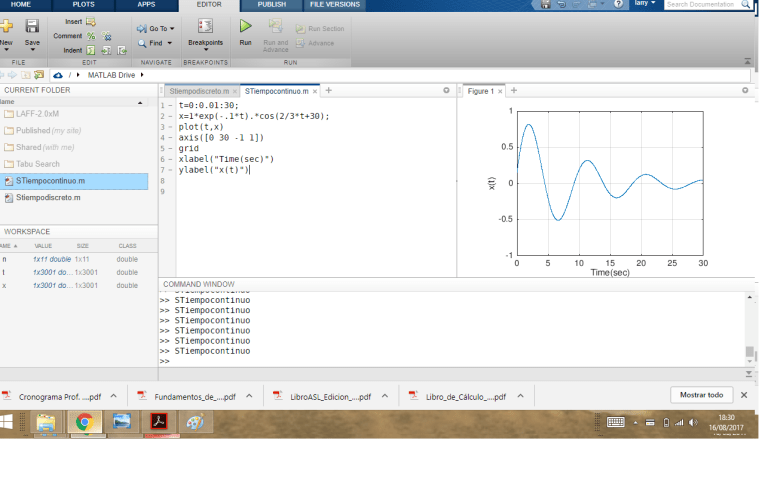
Equation (38) clearly shows what had been observed previously. An example can be simulated in Matlab by the following procedure:
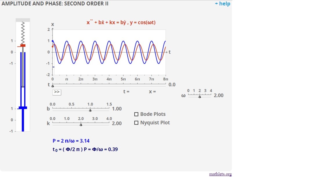
The shape of the displacement curve in a mass-spring-damper system is represented by a sinusoid damped by a decreasing exponential factor. It is important to understand that in the previous case no force is being applied to the system, so the behavior of this system can be classified as «natural behavior» (also called homogeneous response). Later we show the example of applying a force to the system (a unitary step), which generates a «forced behavior» that influences the final behavior of the system that will be the result of adding both behaviors (natural + forced). Remark: When a force is applied to the system, the right side of equation (37) is no longer equal to zero, and the equation is no longer homogeneous.
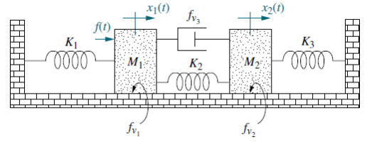
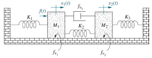
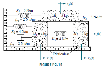
The solution for the equation (37) presented above, can be derived by the traditional method to solve differential equations. However, this method is impractical when we encounter more complicated systems such as the following, in which a force f(t) is also applied:
Figura 7
The need arises for a more practical method to find the dynamics of the systems and facilitate the subsequent analysis of their behavior by computer simulation. The Laplace Transform allows to reach this objective in a fast and rigorous way.
In equation (37) it is not easy to clear x(t), which in this case is the function of output and interest. A differential equation can not be represented either in the form of a Block Diagram, which is the language most used by engineers to model systems, transforming something complex into a visual object easier to understand and analyze.The first step is to clearly separate the output function x(t), the input function f(t) and the system function (also known as Transfer Function), reaching a representation like the following:
r(t)=f(t), c(t)=x(t)
The Laplace Transform consists of changing the functions of interest from the time domain to the frequency domain by means of the following equation:
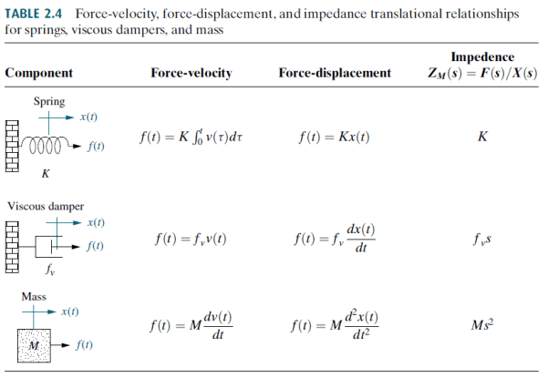
The main advantage of this change is that it transforms derivatives into addition and subtraction, then, through associations, we can clear the function of interest by applying the simple rules of algebra. In addition, it is not necessary to apply equation (2.1) to all the functions f(t) that we find, when tables are available that already indicate the transformation of functions that occur with great frequency in all phenomena, such as the sinusoids (mass system output, spring and shock absorber) or the step function (input representing a sudden change). In the case of our basic elements for a mechanical system, ie: mass, spring and damper, we have the following table:
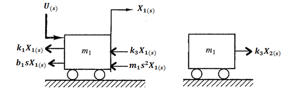
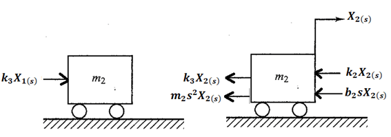
That is, we apply a force diagram for each mass unit of the system, we substitute the expression of each force in time for its frequency equivalent (which in the table is called Impedance, making an analogy between mechanical systems and electrical systems) and apply the superposition property (each movement is studied separately and then the result is added).
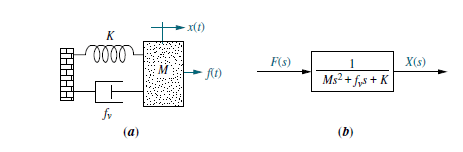
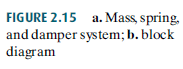
Figure 2.15 shows the Laplace Transform for a mass-spring-damper system whose dynamics are described by a single differential equation:
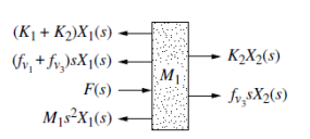
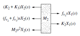
The system of Figure 7 allows describing a fairly practical general method for finding the Laplace Transform of systems with several differential equations. First the force diagram is applied to each unit of mass:
For Figure 7 we are interested in knowing the Transfer Function G(s)=X2(s)/F(s).
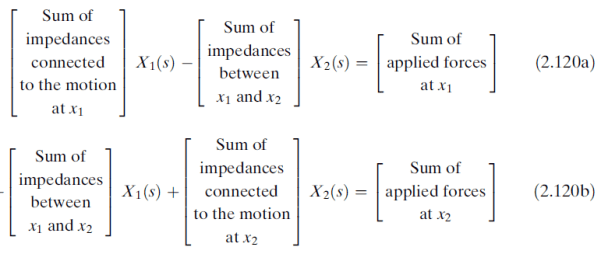
Arranging in matrix form the equations of motion we obtain the following:
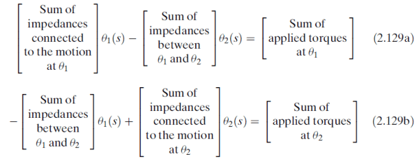
Equations (2.118a) and (2.118b) show a pattern that is always true and can be applied to any mass-spring-damper system:
The immediate consequence of the previous method is that it greatly facilitates obtaining the equations of motion for a mass-spring-damper system, unlike what happens with differential equations. In addition, we can quickly reach the required solution. In the case of our example:
Where:
These are results obtained by applying the rules of Linear Algebra, which gives great computational power to the Laplace Transform method.
Application examples ...under construction
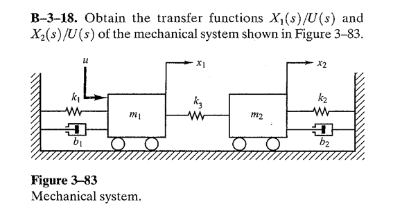
Example 1.
Exercise B318, Modern_Control_Engineering, Ogata 4t p 149 (162),
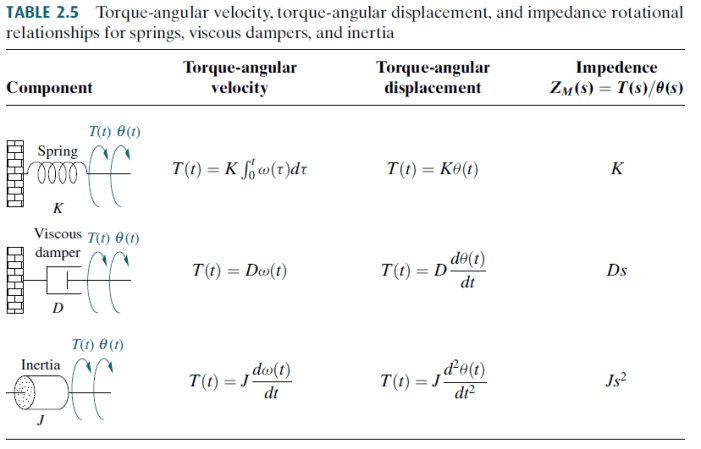
So far, only the translational case has been considered. In the case that the displacement is rotational, the following table summarizes the application of the Laplace transform in that case:
Example:
The following figures illustrate how to perform the force diagram for this case:
Therefore:
Being:
We observe that again it is true that:
Bibliography
:
Robert Resnick, tomo1
Dinamica_de_Sistemas, Katsuhiko Ogata
Control Systems Engineering, Norman Nise
Sistemas de Control Automatico, Benjamin Kuo
Ingenieria de Control Moderna, 3° ED. – Katsuhiko Ogata
Attention!
I recommend the book «Mass-spring-damper system, 73 Exercises Resolved and Explained» I have written it after grouping, ordering and solving the most frequent exercises in the books that are used in the university classes of Systems Engineering Control, Mechanics, Electronics, Mechatronics and Electromechanics, among others.
If you need to acquire the problem solving skills, this is an excellent option to train and be effective when presenting exams, or have a solid base to start a career on this field.
INDEX
Preface ii
Introduction iii
Chapter 1———————————————————- 1
o Mass-spring-damper System (translational mechanical system)
Chapter 2———————————————————- 51
o Mass-spring-damper System (rotational mechanical system)
Chapter 3———————————————————- 76
o Mechanical Systems with gears
Chapter 4———————————————————- 89
o Electrical and Electronic Systems
Chapter 5——————————————————— 114
o Electromechanical Systems – DC Motor
Chapter 6——————————————————— 144
o Liquid level Systems
Chapter 7——————————————————— 154
o Linearization of nonlinear Systems
References——————————————————- 164
Attention!
If what you need is to determine the Transfer Function of a System … We deliver the answer in two hours or less, depending on the complexity. In digital Contact us, immediate response, solve and deliver the transfer function of mass-spring-damper systems, electrical, electromechanical, electromotive, liquid level, thermal, hybrid, rotational, non-linear, etc. Optional, Representation in State Variables. Simulation in Matlab, Optional, Interview by Skype to explain the solution.
WhatsApp +34633129287, Inmediate attention !!
email: dademuchconnection@gmail.com
Written by Prof. Larry Francis Obando – Technical Specialist – Educational Content Writer
Mentoring Académico / Emprendedores / Empresarial
Copywriting, Content Marketing, Tesis, Monografías, Paper Académicos, White Papers (Español – Inglés)
Escuela de Ingeniería Electrónica de la Universidad Simón Bolívar, USB Valle de Sartenejas.
Escuela de Ingeniería Eléctrica de la Universidad Central de Venezuela, UCV CCs
Escuela de Turismo de la Universidad Simón Bolívar, Núcleo Litoral.
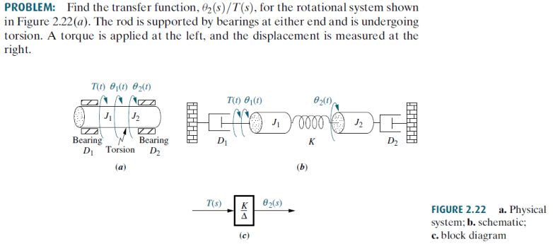
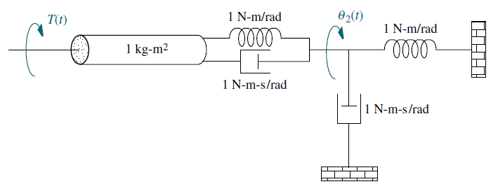
Determinar la Función de Transferencia, G(s)=θ2(s)/T(s), para el sistema mecánico rotacional mostrado en la Figura 2.26 (Nise):
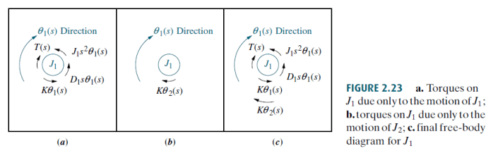
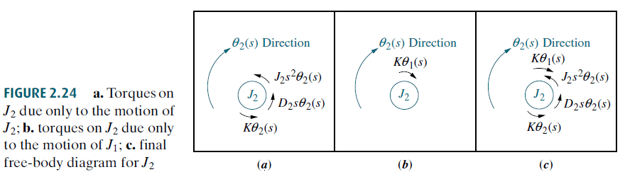
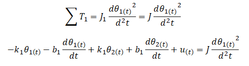
1. Dinámica del sistema:
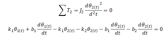
Por otra parte:
2. Transformada de Laplace:
Ecuación 1:
Ecuación 2:
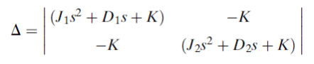
3. Función de Transferencia:
Sustituyendo los valores:
De dónde:
Control Systems Engineering, Norman Nise
Sistemas de Control Automatico, Benjamin Kuo
Ingenieria de Control Moderna, 3° ED. – Katsuhiko Ogata
Revisión literaria hecha por:
Prof. Larry Francis Obando – Technical Specialist – Educational Content Writer
La realimentación electrónica consiste en tomar la información disponible en una parte del circuito e introducirla en otra parte del circuito con el fin de influir sobre el comportamiento de la salida.
La realimentación, o feedback (fb), es un concepto físico y no un concepto matemático, e implica un gasto de energía. Por tanto, la energía disponible en el origen de la información debe ser superior a la energía en el punto destino. Es por ello que se requiere de un circuito electrónico para poder implementar una realimentación efectiva, debido a que este tipo de circuitos permite incrementar la energía de la información a medida que ésta fluye a través del sistema, además de que permite establecer un flujo de información con dirección contraria a la que dicho flujo tiene debido a la naturaleza e influencia del sistema.
Ojo, no sólo los sistemas electrónicos son capaces de implementar un sistema realimentado. Existen numerosos mecanismos de realimentación que forman parte de nuestra vida cotidiana. El tanque de la poceta tradicional se llena de agua hasta que el nivel de líquido empuja un globo que acciona un pistón cerrando el surtidor de agua. Éste es un sistema realimentado donde el nivel de líquido es la información dirigida a la entrada, el pistón que controla el surtidor. Pero el uso de la electrónica tiene ventajas, como de la reducción de costos en términos monetarios y de espacio, o la estética.
El objetivo fundamental de la realimentación electrónica, sin embargo, es modificar la salida del sistema y hacerla lo más independiente posible de los parámetros internos del mismo sistema. Este mecanismo permite controlar el sistema. De hecho, se requieren tantas líneas de realimentación como variables que se deseen controlar.
Estructura general de un circuito realimentado
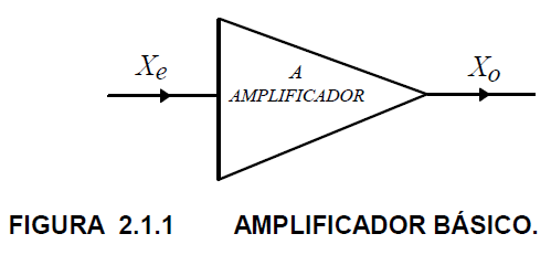
Para representar la estructura básica de un sistema electrónico realimentado utilizaremos el amplificador de la Figura 2.1.1:
Se aplica una señal de entrada Xe al amplificador A, la cual puede ser un voltaje o una corriente. Xo representa la salida del amplificador. Supongamos que Xe y Xo tienen las mismas dimensiones, o unidades.
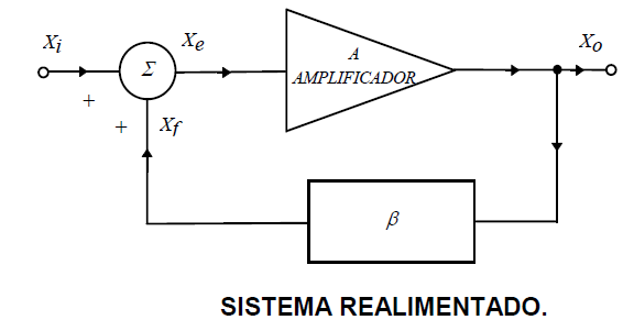
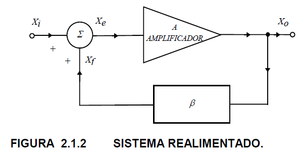
Al implementar un circuito realimentado básico, debemos transportar información desde la salida a la entrada, con el fin de sumar o comparar ambas señales, tal como se muestra en la Figura 2.1.2:
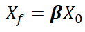
En la Figura anterior podemos identificar claramente tres estructuras representadas por tres bloques: un amplificador A, un circuito de transferencia β, y un sumador. El bloque A amplifica la señal incrementado la energía de la información. El bloque β transfiere la información de la salida a una de las entradas del sumador, cuya función puede ser sumar o restar esta señal a la entrada. El sumador suma o resta las señales Xi y Xf, que provienen de la entrada y salida del bloque β respectivamente, generando una señal Xe. A continuación, vamos a obtener una expresión matemática para la ganancia del sistema Xo/Xi.
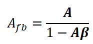
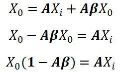
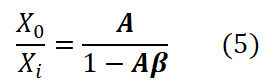
Sabemos del estudio de amplificadores operacionales que la salida Xo puede ser expresada en términos de la ganancia A como:Donde Xe no es la entrada al sistema sino la entrada al amplificador y es igual a:Al sustituir la ecuación (2) en (1):Dónde:Por tanto:Luego:Por tanto: La ecuación (5) es una de las más importantes de la ingeniería electrónica y se le denomina en la literatura general como Ganancia del sistema realimentado o Ganancia a lazo cerrado. Fue el ingeniero Harold Black en 1928 quién primero utilizó la denotación Afb para esta ganancia. Por tanto:
Comportamiento de un circuito realimentado
En construcción…
Referencia: ANALISIS DE SISTEMAS ELECTRONICOS
Escrito por: Profesor Larry Obando – Technical Specialist – Educational Content Writer.
Mentoring Académico / Empresarial / Emprendedores
Copywriting, Content Marketing, Tesis, Monografías, Paper Académicos, White Papers (Español – Inglés)
Escuela de Ingeniería Eléctrica de la Universidad Central de Venezuela, Caracas.
Escuela de Ingeniería Electrónica de la Universidad Simón Bolívar, Valle de Sartenejas.
Escuela de Turismo de la Universidad Simón Bolívar, Núcleo Litoral.
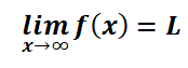
Sea f una función definida en [c,∞) para algún número c. Decimos que:
Si para cada ε>0, existe un correspondiente número M, tal que:
Límite cuando x→-∞
Sea f una función definida en (-∞, c] para algún número c. Decimos que:
Si para cada ε>0, existe un correspondiente número M, tal que:
Ejemplo 1. Demostrar que:
Solución. Por lo general se utiliza un truco común: dividir el numerador y el denominador entre la potencia más alta de x que aparece en el denominador, que en este caso es 2:Ejemplo 2. Encuentre:Solución:
Por tanto:Ejemplo 3. Encuentre:Solución:Por tanto:
Escrito por: Profesor Larry Obando – Technical Specialist – Educational Content Writer.
Mentoring Académico / Empresarial / Emprendedores
Copywriting, Content Marketing, Tesis, Monografías, Paper Académicos, White Papers (Español – Inglés)
Escuela de Ingeniería Eléctrica de la Universidad Central de Venezuela, Caracas.
Escuela de Ingeniería Electrónica de la Universidad Simón Bolívar, Valle de Sartenejas.
Escuela de Turismo de la Universidad Simón Bolívar, Núcleo Litoral.
Die Grundelemente eines jeden mechanischen Systems sind die Masse, die Feder und der Stoßdämpfer. Das Studium der Bewegung in mechanischen Systemen entspricht der Analyse dynamischer Systeme. In der Robotik zum Beispiel bezieht sich das Wort Vorwärtsdynamik darauf, was mit Aktuatoren passiert, wenn wir bestimmte Kräfte und Drehmomente auf sie anwenden.
Die Masse, die Feder, der Stoßdämpfer sind elementare Aktuatoren eines mechanischen Systems.
Um den Roboter zu steuern, ist es folglich notwendig, die Art der Bewegung eines Masse-Feder-Dämpfer-Systems sehr gut zu kennen.
Darüber hinaus wird dieses elementare System in vielen Anwendungsbereichen vorgestellt, daher die Wichtigkeit seiner Analyse. Wenn wir in der Robotik über Inverse Dynamic sprechen, sprechen wir darüber, wie man den Roboter auf eine gewünschte Art und Weise bewegt, welche Kräfte und Drehmomente wir auf die Aktoren anwenden müssen, damit sich unser Roboter auf eine bestimmte Art bewegt.
Bevor wir die dynamische Analyse unseres Masse-Feder-Dämpfer-Systems durchführen, müssen wir sein mathematisches Modell erhalten. Dies ist der erste Schritt für jeden, der die Dynamik eines Systems, insbesondere das Verhalten seiner mechanischen Komponenten, genau kennenlernen möchte.
Wir werden unsere Studie mit dem Modell eines Masse-Feder-Systems beginnen.
Dies ist aus folgendem Grund praktisch. Alle mechanischen Systeme haben eine Art in ihrer Bewegung, die sie zum Schwingen bringt, etwa wenn ein Gegenstand an einem Faden an der Decke hängt und mit der Hand, die wir drücken. Oder ein Schuh auf einer Plattform mit Federn. Es ist gut zu wissen, welche mathematische Funktion diese Bewegung am besten beschreibt.
Masse-Feder-System.
Abbildung 5
Die Dynamik eines Systems wird in erster Linie durch ein mathematisches Modell dargestellt, das aus Differentialgleichungen besteht. Im Falle des Masse-Feder-Systems ist diese Gleichung wie folgt:
Diese Gleichung ist als Bewegungsgleichung eines einfachen harmonischen Oszillators bekannt. Mal sehen, woher es stammt.
Wenn wir eine Formel erhalten wollen, die die Kraft beschreibt, die eine Feder gegen die Verschiebung ausübt, die sie dehnt oder schrumpft, ist es am besten, die potentielle Energie zu visualisieren, die in die Feder injiziert wird, wenn wir sie dehnen oder schrumpfen. Die folgende Grafik beschreibt, wie sich diese Energie als Funktion der horizontalen Verschiebung verhält:
Wenn sich die Masse m der vorhergehenden Figur, die an dem Ende der Feder angebracht ist, wie in Abbildung 5 gezeigt, von dem Federrelaxationspunkt x = 0 weg in die positive oder negative Richtung bewegt, sammelt sich die potentielle Energie U (x)an und steigt in parabolischer Form an und erreicht einen höheren Energiewert, wobei U(x) = E, Wert, der der maximalen Dehnung oder Kompression der Feder entspricht. Die mathematische Gleichung, die in der Praxis diese Kurvenform am besten beschreibt und eine Konstante k für die physikalische Eigenschaft des Materials enthält, die die Steigung der Kurve erhöht oder verringert, ist die folgende:
Die Kraft ist auf folgende Weise mit der potentiellen Energie verbunden:
Deshalb:
Es ist sinnvoll zu sehen, dass F (x) umgekehrt proportional zur Verschiebung der Masse m ist. Denn es ist klar, dass, wenn wir die Feder dehnen oder schrumpfen, diese Kraft dieser Aktion entgegenwirkt und versucht, die Feder in ihre entspannte oder natürliche Position zurückzubringen. Aus diesem Grund heißt es Restitutionskraft. Die obige Gleichung ist in der Akademie als Hookes Gesetz oder Kraftgesetz für Federn bekannt. Das Folgende ist ein repräsentatives Diagramm dieser Kraft in Bezug auf die Energie, wie sie erwähnt wurde, ohne den Eingriff von Reibungskräften (Dämpfung), weshalb sie als der einfache harmonische Oszillator bekannt ist. Es ist wichtig, die proportionale Beziehung zwischen Verschiebung und Kraft zu betonen, aber mit einer negativen Steigung, und das ist in der Praxis komplexer, nicht linear.
Diese Gleichung sagt uns, dass die vektorielle Summe aller Kräfte, die auf den Körper der Masse m einwirken, gleich dem Produkt des Wertes der Masse aufgrund ihrer Beschleunigung ist, die aufgrund der Kräfte erhalten wird. Mit Newtons zweitem Gesetz erhalten wir die folgende Gleichung:
Das ist:
Diese Gleichung repräsentiert die Dynamik eines idealen Masse-Feder-Systems.
System Masse-Feder-Stoßdämpfer
Wenn keine Reibungskraft vorhanden ist, oszilliert der einfache harmonische Oszillator unendlich. In Wirklichkeit nimmt die Amplitude der Oszillation allmählich ab, ein Prozess, der als Dämpfung bekannt ist und im folgenden graphisch beschrieben wird:
Die Verschiebung einer oszillierenden Bewegung ist gegen die Zeit aufgetragen, und ihre Amplitude wird durch eine sinusförmige Funktion dargestellt, die durch einen abnehmenden Exponentialfaktor gedämpft wird, der in dem Graphen als eine Hüllkurve erscheint. Die Reibungskraft Fv, die auf die amortisierte harmonische Bewegung einwirkt, ist in den meisten Fällen von wissenschaftlichem Interesse proportional zur Geschwindigkeit V. Diese Kraft hat die Form Fv = bV, wobei b eine positive Konstante ist, die unter anderem von den Eigenschaften des Fluids abhängt, das Reibung verursacht. Diese Reibung, auch bekannt als Viskosereibung, wird durch ein Diagramm dargestellt, das aus einem Kolben und einem mit Öl gefüllten Zylinder besteht:
Die gängigste Art, ein Masse-Feder-Dämpfer-System darzustellen, ist eine Reihenschaltung wie folgt:
Abbildung 6
Sowie die folgenden:
In beiden Fällen wird das gleiche Ergebnis bei Anwendung unserer Analysemethode erhalten. Wenn man Fig. 6 betrachtet, kann man sehen, dass dieselbe Konfiguration wie in Fig. 5 gezeigt ist, jedoch die Wirkung des Stoßdämpfers hinzugefügt wird. Indem wir Newtons zweites Gesetz auf dieses neue System anwenden, erhalten wir die folgende Beziehung:
Diese Gleichung repräsentiert die Dynamik eines Massen-Feder-Schock-Systems.
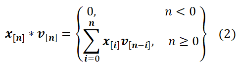
Dadas dos señales de tiempo discreto x[n] y v[n], la convolución de ambas señales se define como:
La expresión del lado derecho de la ecuación (1) se conoce como sumatoria de convolución. En el caso de que ambas señales x[n] y v[n] sean iguales a cero para n<0, entonces x[i]=0 para i<0, y v[n-i]=0 para n-i<0, entonces la ecuación (1) se puede escribir como:
Ejemplos
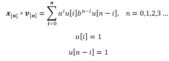
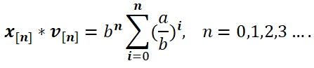
Suponiendo que x[n]=anu[n], donde u[n] es la función escalón, y v[n]= bnu[n]. La convolución entre ambas señales es igual a:
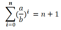
Si a=b:Entonces:
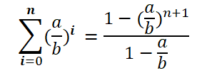
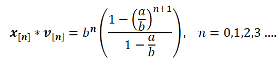
Si a ≠b:
Por tanto:
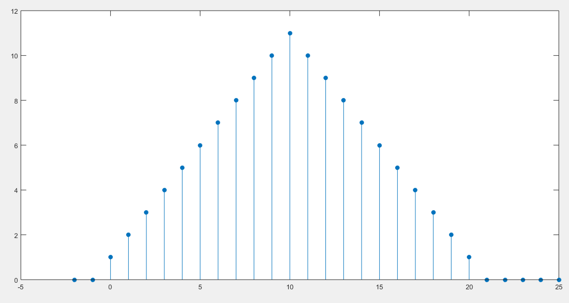
2. La convolución de dos señales discretas puede representarse en Matlab mediante el siguiente código. Por ejemplo, la convolución de una señal p[n] consigo misma:
>> p=[0 ones(1,11) zeros(1,5)]%correspondiente a n=-1 a n=14
>>x=p
>> v=p
>> y=conv(x,v)
>> n=-2:25;
>> stem(n,y(1:length(n)),’filled’)
Convolución de una señal (p{n]=1 ) consigo misma.
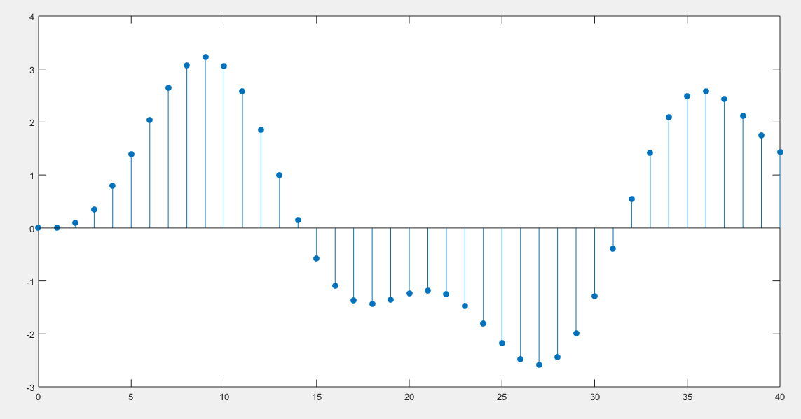
3. Si aplicamos la convolución entre una entrada discreta x[n] a un sistema y la respuesta h[n] al impulso unitario discretode dicho sistema, obtendremos la salida. Si h[n]=sen(0.5n) para n ≥0, y la entrada x[n]=sen(0.2n) para n ≥0, podemos representar la salida mediante Matlab como sigue:
>> n=0:40;
>> x=sin(.2*n);
>> h=sin(.5*n);
>>y=conv(x,h);
>> stem(n,y(1:length(n)),’filled’)
Salida y[n] para el sistema con entrada x[n]=sen(0.2n) y respuesta al impulso h[n]=sen(0.5n)ANTERIOR:
Si lo que Usted necesita es resolver con urgencia un problema:
Atención:
Si lo que Usted necesita es determinar La Función de Transferencia de un Sistema..Le entregamos la respuesta en dos horas o menos, dependiendo de la complejidad. En digital. Póngase en contacto con nosotros, respuesta inmediata, resolvemos y entregamos la Función de Transferencia de sistemas masa-resorte-amortiguador, eléctricos, electromecánicos, electromotriz, nivel de líquido, térmico, híbridos, rotacional, no lineales, etc.. Opcional, Representación en Variables de Estado. Opcional, Entrevista por Skype para explicar la solución.



















 1.
1.  Por otra parte:
 2.
2.  Ecuación 2:
 3. Función de Transferencia:
 Sustituyendo los valores:
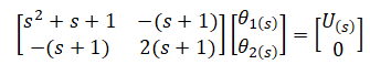
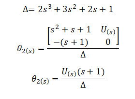 De dónde:

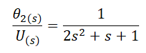
 Donde Xe no es la entrada al sistema sino la entrada al amplificador y es igual a:
 Al sustituir la ecuación (2) en (1):
 Dónde:
 Por tanto:
 Luego:
 Por tanto:
  La ecuación (5) es una de las más importantes de la ingeniería electrónica y se le denomina en la literatura general como Ganancia del sistema realimentado o Ganancia a lazo cerrado. Fue el ingeniero Harold Black en 1928 quién primero utilizó la denotación Afb para esta ganancia. Por tanto: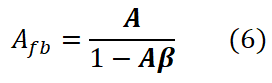
 Si para cada ε>0, existe un correspondiente número M, tal que:
 Límite cuando x→-∞
 Ejemplo 1. Demostrar que: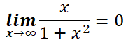
 Ejemplo 2. Encuentre:
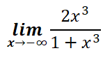 Solución:
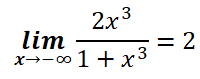 Ejemplo 3. Encuentre:
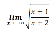 Solución:
 Por tanto: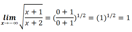



 Si a=b:
 Entonces:

 dademuchconnection