Base de conocimiento

Computer Science, UML

UML Analysis – Basics

Computer science and programming

Jueves 09 noviembre, 09:44 am

Fuente:

Object-Oriented Software Engineering

    1. Analysis p 173
    2. Overview of Analysis
    3. Analysis Concepts pp 176
    4. Analysis Activities pp 179

Analysis

Analysis results in a model of the system that aims to be correct, complete, consistent, and unambiguous. Developers formalize the requirements specification produced during requirements elicitation and examine in more detail boundary conditions and exceptional cases. Developers validate, correct and clarify the requirements specification if any errors or ambiguities are found. The client and the user are usually involved in this activity when the requirements specification must be changed and when additional information must be gathered. In object-oriented analysis, developers build a model describing the application domain.

Formalization helps identify areas of ambiguity as well as inconsistencies and omissions in a requirements specification. Once developers identify problems with the specification, the address them by eliciting more information from the users and the client. Requirements elicitation and analysis are iterative and incremental activities that occur concurrently.

An Overview of Analysis

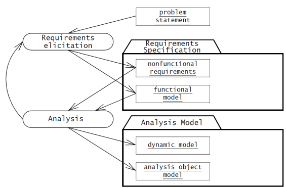
Analysis focuses on producing a model of the system, called the analysis model, which is correct, complete, consistent, and verifiable. Analysis is different from requirements elicitation in that developers focus on structuring and formalizing the requirements elicited from users (Figure 5-2).
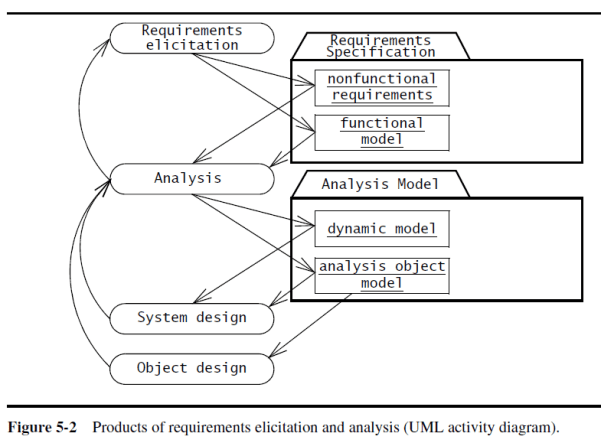
This formalization leads to new insights and the discovery of errors in the requirements. As the analysis model may not be understandable to the users and the client, developers need to update the requirements specification to reflect insights gained during analysis, then review the changes with the client and the users. In the end, the requirements, however large, should be understandable by the client and the users.

The analysis model is composed of three individual models: the functional model, represented by use cases and scenarios, the analysis object model, represented by class and object diagrams, and the dynamic model, represented by state machine and sequence diagrams (Figure 5-3).
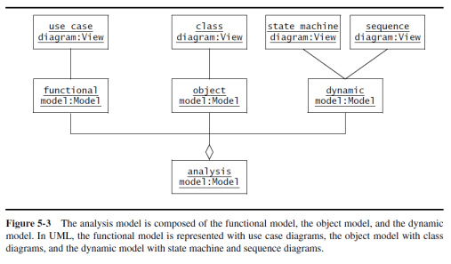
In the previous chapter, we described how to elicit requirements from the users and describe them as use cases and scenarios. In this chapter, we describe how to refine the functional model and derive the object and the dynamic model. This leads to a more precise and complete specification as details are added to the analysis model.

Analysis Object Model

The analysis model represents the system under development from the user’s point of view. The analysis object model is a part of the analysis model and focuses on the individual concepts that are manipulated by the system, their properties and their relationships. The analysis object model, depicted with UML class diagrams, includes classes, attributes, and operations. The analysis object model is a visual dictionary of the main concepts visible to the user.

Dynamic Model

The dynamic model focuses on the behavior of the system. The dynamic model is depicted with sequence diagrams and with state machines. Sequence diagrams represent the interactions among a set of objects during a single use case. State machines represent the behavior of a single object (or a group of very tightly coupled objects). The dynamic model serves to assign responsibilities to individual classes and, in the process, to identify new classes, associations, and attributes to be added to the analysis object model.

Entity, Boundary, and Control Objects

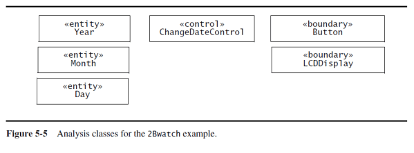
The analysis object model consists of entity, boundary, and control objects [Jacobson et al., 1999]. Entity objects represent the persistent information tracked by the system. Boundary objects represent the interactions between the actors and the system. Control objects are in charge of realizing use cases. In the 2Bwatch example, Year, Month, and Day are entity objects; Button and LCDDisplay are boundary objects; ChangeDateControl is a control object that represents the activity of changing the date by pressing combinations of buttons.Modeling the system with entity, boundary, and control objects provides developers with simple heuristics to distinguish different, but related concepts.

To distinguish between different types of objects, UML provides the stereotype mechanism to enable the developer to attach such meta-information to modeling elements.

For example, in Figure 5-5, we attach the «control» stereotype to the ChangeDateControl object. In addition to stereotypes, we may also use naming conventions for clarity and recommend distinguishing the three different types of objects on a syntactical basis: control objects may have the suffix Control appended to their name; boundary objects may be named to clearly denote an interface feature (e.g., by including the suffix Form, Button, Display, or Boundary); entity objects usually do not have any suffix appended to their name.
Generalization and Specialization

Modeling with UML, inheritance enables us to organize concepts into hierarchies. At the top of the hierarchy is a general concept, and at the bottom of the hierarchy are the most specialized concepts.

Generalization is the modeling activity that identifies abstract concepts from lower-level ones.

Specialization is the activity that identifies more specific concepts from a high-level one.
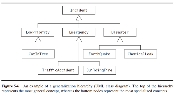
In some instances, modelers call inheritance relationships generalization-specialization relationships. In this book, we use the term “inheritance” to denote the relationship and the terms “generalization” and “specialization” to denote the activities that find inheritance relationships.

Analysis Activities: From Use Cases to Objects

In this section, we describe the activities that transform the use cases and scenarios produced during requirements elicitation into an analysis model. Analysis activities include:

  1. Identifying Entity Objects
  2. Identifying Boundary Objects
  3. Identifying Control Objects
  4. Mapping Use Cases to Objects with Sequence Diagrams
  5. Modeling Interactions among Objects with CRC Cards
  6. Identifying Associations
  7. Identifying Aggregates
  8. Identifying Attributes
  9. Modeling State-Dependent Behavior of Individual Objects
  10. Modeling Inheritance Relationships
  11. Reviewing the Analysis Model

Identifying Entity Objects

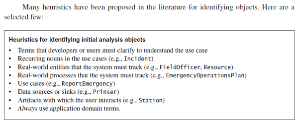
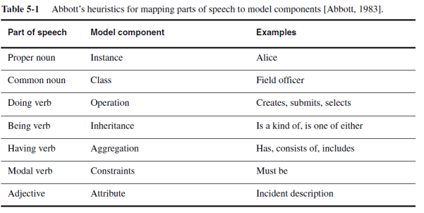
Participating objects form the basis of the analysis model. Natural language analysis is an intuitive set of heuristics for identifying objects, attributes, and associations from a requirements specification. Abbott’s heuristics maps parts of speech (e.g., nouns, having verbs, being verbs, adjectives) to model components (e.g., objects, operations, inheritance relationships, classes). Table 5-1 provides examples of such mappings by examining the ReportEmergency use case:
The following heuristics can be used in conjunction with Abbott’s heuristics:
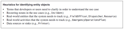
As it was mentioned before, Entity Objects represent the persistent information tracked by the system. For entity objects we recommend always to start with the names used by end users and application domain specialists. Describing objects, even briefly, allows developers to clarify the concepts they use and avoid misunderstandings (e.g., using one object for two different but related concepts).

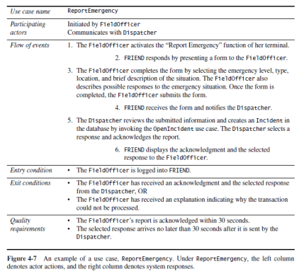
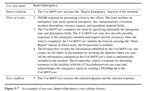
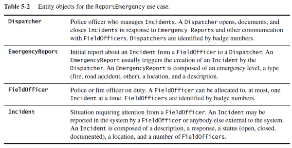
For example, after a first examination of the ReportEmergency use case (Figure 5-7), we use application domain knowledge and interviews with the users to identify the objects Dispatcher, EmergencyReport, FieldOfficer, and Incident. Note that the EmergencyReport object is not mentioned explicitly by name in the ReportEmergency use case. Step 4 of the use case refers to the emergency report as the “information submitted by the FieldOfficer.” After review with the client, we discover that this information is usually referred to as the “emergency report” and decide to name the corresponding object EmergencyReport.
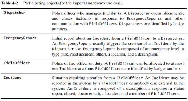
The definition of entity objects leads to the initial analysis model described in Table 5-2.
Identifying Boundary Objects

Boundary objects represent the system interface with the actors. In each use case, each actor interacts with at least one boundary object. The boundary object collects the information from the actor and translates it into a form that can be used by both entity and control objects.
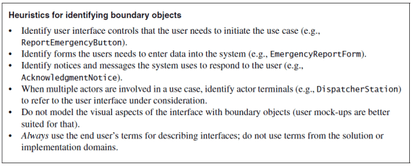
We find the boundary objects of Table 5-3 by examining the ReportEmergency use case.
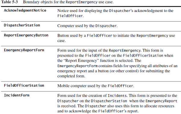
We have made progress toward describing the system. We now have included the interface between the actor and the system. We are, however, still missing some significant pieces of the description, such as the order in which the interactions between the actors and the system occur. In the next section, we describe the identification of control objects.

Identifying Control Objects

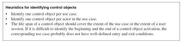
Control objects are responsible for coordinating boundary and entity objects. Control objects usually do not have a concrete counterpart in the real world. Often a close relationship exists between a use case and a control object; a control object is usually created at the beginning of a use case and ceases to exist at its end. It is responsible for collecting information from the boundary objects and dispatching it to entity objects. For example, control objects describe the behavior associated with the sequencing of forms, undo and history queues, and dispatching information in a distributed system.

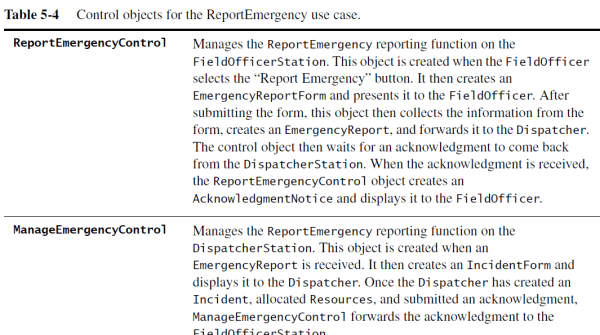
We model the control flow of the ReportEmergency use case with a control object for each actor: ReportEmergencyControl for the FieldOfficer and ManageEmergency-Control for the Dispatcher, respectively (Table 5-4).

The decision to model the control flow of the ReportEmergency use case with two control objects stems from the knowledge that the FieldOfficerStation and the DispatcherStation are actually two subsystems communicating over an asynchronous link.
Literature Review by: Larry Francis Obando – Technical Specialist

Escuela de Ingeniería Eléctrica de la Universidad Central de Venezuela, Caracas.

Escuela de Ingeniería Electrónica de la Universidad Simón Bolívar, Valle de Sartenejas.

Escuela de Turismo de la Universidad Simón Bolívar, Núcleo Litoral.

Contact: Caracas, Valladolid, Quito, Guayaquil, Jaén, Villafranca de Ordizia

WhatsApp: +34633129287

00593984950376

email: dademuchconnection@gmail.com
Diodos y circuitos con diodos, Electronic Engineer

Diodos – Caracteres básicos

Diodos – Caracteres básicos.

Jueves 09 de noviembre, 2017, 04:43 am.

Fuente:

  1. Electrónica Hambley
    1. Características del diodo pp 137-145 (148)

Características del diodo.

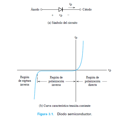
El diodo es un dispositivo electrónico de gran importancia, que posee dos terminales: el ánodo y el cátodo. El símbolo del diodo se muestra en la Figura 3.1(a), mientras que en la Figura 3.1(b) se muestra su característica tensión-corriente.

La tensión vD en el diodo se toma como positiva de ánodo a cátodo. De igual manera, la corriente iD en el diodo se referencia como positiva cuando circula de ánodo a cátodo.

Puede observarse en la curva característica que, si la tensión vD es positiva en el diodo, pasa un flujo de corriente grande incluso con pequeñas tensiones. Esta condición se denomina polarización directa. Así, la corriente fluye fácilmente a través del diodo en la dirección que indica la flecha o el símbolo del diodo.

Por otra parte, para valores moderadamente negativos de vD, la corriente iD es muy pequeña. A esto se le llama región de polarización inversa, como puede verse en la curva característica del diodo. Si se aplica una tensión de polarización inversa suficientemente grande al diodo, su modo de operación entra en la región de ruptura inversa o zona de avalancha, permitiendo el flujo de una elevada corriente.

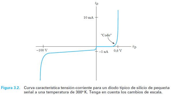
En la Figura 3.2 se muestra la curva característica de un diodo típico de silicio de pequeña señal trabajando a una temperatura de 300o K. Observe que las escalas para la tensión y la corriente en la región de polarización directa son diferentes a las utilizadas en la región de polarización inversa. Esto ayuda a presentar con claridad los detalles de la curva característica ya que los valores de corriente son mucho más pequeños, y los de tensión mucho más grandes, en la región de polarización inversa que en la región de polarización directa.

Los diodos de silicio de pequeña señal se pueden encontrar comúnmente en circuitos electrónicos de baja y media potencia. Uno de esos diodos discretos es el 1N4148, distribuido por varios fabricantes. Los diodos en los circuitos integrados tienen características similares a las de los diodos discretos de pequeña señal.

En la región de polarización directa, los diodos de silicio de pequeña señal conducen muy poca corriente (mucho menos de 1 mA), hasta que se aplica una tensión directa de 0,6 a 0,7 V (suponiendo que el diodo se encuentra a una temperatura de aproximadamente 300o K). Entonces, la corriente aumenta muy rápidamente a medida que se sigue incrementando la tensión. Decimos que la curva característica de polarización directa presenta un codo sobre los 0,6 V. A medida que aumenta la temperatura, la tensión de codo disminuye a razón de aproximadamente 2 mV/K.

En la región de polarización inversa, para diodos de silicio de pequeña señal a temperatura ambiente, la corriente típica es de, aproximadamente, 1 nA. Cuando se alcanza la ruptura inversa, la corriente aumenta de valor rápidamente. La tensión para la que ocurre esto se llama tensión de ruptura. Por ejemplo, la tensión de ruptura de la curva característica del diodo mostrada en la Figura 3.2 es, aproximadamente, de -100 V.

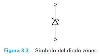
Los diodos que trabajan en la zona de ruptura se denominan diodos zéner o diodos de avalancha. Los diodos zéner se usan en aplicaciones para las que se necesita una tensión constante en la región de ruptura. Por tanto, los fabricantes intentan optimizar los diodos zéner para obtener una curva característica prácticamente vertical en la región de ruptura. El símbolo modificado del diodo que se muestra en la Figura 3.3 es el que se usa para los diodos zéner.


Análisis de la línea de carga.

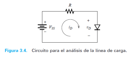
La curva característica tensión-corriente de los diodos no es lineal. A causa de esta no linealidad, muchas de las técnicas aprendidas en los cursos básicos de teoría de circuitos para trabajar con circuitos lineales no se pueden aplicar a circuitos que empleen diodos. Los métodos gráficos constituyen un enfoque para analizar este tipo de circuitos. Por ejemplo, consideremos el circuito de la Figura 3.4.

Aplicando la ley de tensiones de Kirchhoff, podemos escribir:

Supongamos que los valores de VSS y de R se conocen, y que deseamos hallar iD y vD. Así, la Ecuación (3.1) tiene dos incógnitas, por lo que se necesita otra relación entre iD y vD para hallar una solución. La relación necesaria se ve de forma gráfica en la Figura 3.5, en la que se muestra la curva característica tensión-corriente del diodo.

Podemos obtener la solución trazando la Ecuación (3.1) en los mismos ejes que la curva característica del diodo. El punto de trabajo es la intersección de la línea de carga y la curva característica del diodo. El punto de trabajo representa la solución simultánea de la Ecuación (3.1) y de la característica del diodo.

Ejemplos 3.1 y 3.2

Modelo de diodo ideal.

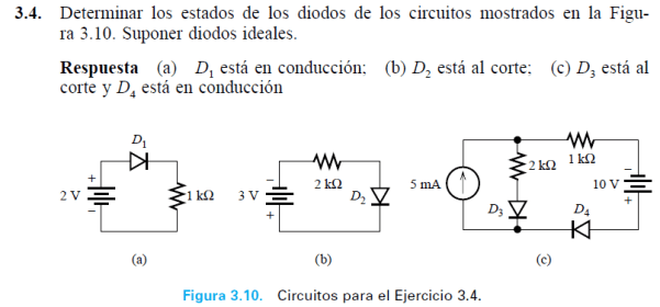
Aunque el análisis de la línea de carga de los circuitos con diodos nos proporciona resultados precisos y reveladores, necesitamos modelos más simples para analizar con rapidez circuitos que contengan varios diodos. Un modelo muy útil para ello es el modelo del diodo ideal, un conductor perfecto con una caída de tensión cero en conducción directa. En conducción inversa, el diodo ideal es un circuito abierto. La curva característica tensión – corriente del diodo ideal se muestra en la Figura 3.8.

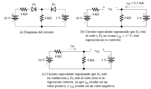
Al analizar un circuito con diodos ideales, puede que inicialmente no sepamos qué diodos están en conducción y cuáles al corte. Por tanto, nos vemos forzados a aventurar condiciones. Luego, analizamos el circuito para encontrar las corrientes en los diodos que hemos supuesto que están en conducción, y las tensiones en los que hemos supuesto que están al corte. Si iD es positiva en los diodos supuestamente en conducción y si vD es negativa en los supuestamente al corte, nuestras presunciones son correctas, y ya hemos resuelto el circuito (estamos suponiendo que iD se referencia como positiva en conducción directa y vD es positiva en el ánodo). Si no es así, debemos hacer otros supuestos respecto a los diodos y comenzar de nuevo. Después de algo de práctica, nuestra primera presunción será casi siempre correcta, al menos en circuitos simples.

Ejemplos 3.3 y 3.4

Literature Review by: Larry Francis Obando – Technical Specialist

Escuela de Ingeniería Eléctrica de la Universidad Central de Venezuela, Caracas.

Escuela de Ingeniería Electrónica de la Universidad Simón Bolívar, Valle de Sartenejas.

Escuela de Turismo de la Universidad Simón Bolívar, Núcleo Litoral.

Contact: Ecuador (Quito, Guayaquil, Cuenca)

WhatsApp: 00593984950376

email: dademuchconnection@gmail.com
Conversión Electromecánica de energía, Máquinas Eléctricas

Concepto de Campo Magnético – Teorema de Gauss

El campo magnético es un modelo que permite describir matemáticamente la influencia magnética de las corrientes eléctricas o de los materiales ferromagnéticos, los cuáles son materiales imanados espontáneamente.

null

Producción de un campo magnético

La ley básica que gobierna la producción de un campo magnético es la ley de Ampere, que relaciona un campo magnético estático de intensidad H, alrededor de un contorno cerrado C, con su causa, es decir, una corriente eléctrica estática de densidad J:

null

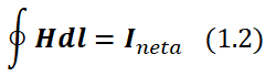
La ecuación 1.1 establece entonces que la fuente del campo magnético H es la densidad de corriente J. El último término es la corriente de desplazamiento. Este término es de gran importancia para los campos magnéticos que se generan en el espacio mediante campos eléctricos variantes en el tiempo, asociados con la radiación electromagnética. Ignorar este término da como resultado un imán cuasiestático, y la ecuación 1.1 se puede simplificar hasta llegar a la ecuación 1.2:

null

Donde H es la intensidad del campo magnético producida por la corriente Ineta, mientras que dl es el elemento diferencial a lo largo de la trayectoria de integración.

Densidad de flujo magnético

Por otra parte, la magnitud física que caracteriza al vector que representa al campo magnético, recibe el nombre de vector de inducción magnética B (también denominado densidad de flujo magnético B), donde:

null

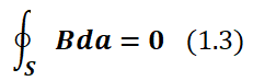
La ecuación 1.3, también conocido como Teorema de Gauss, establece que se conserva la cantidad de flujo magnético, es decir, que ningún flujo magnético neto entra o sale de una superficie cerrada S. Las líneas de flujo magnético sólo existen en lazos continuos, no tienen principio ni fin como es el caso de las líneas de flujo eléctrico. De esta ecuación también se advierte que las cantidades de campo magnético sólo pueden ser determinadas a partir de los valores instantáneos de las fuentes de corriente.

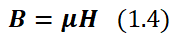
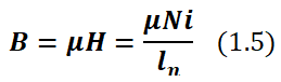
La relación entre el campo magnético y la inducción magnética creada por un material ferromagnético, reviste una importancia extraordinaria en la utilización técnica de dicho material. La inducción magnética B se induce por La intensidad del campo magnético H. La relación entre ambas cantidades es la siguiente:

null

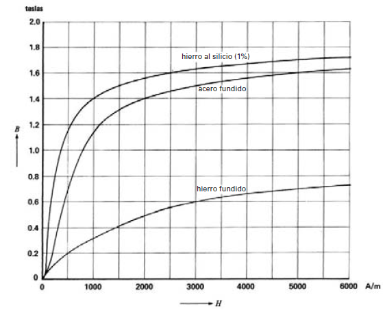
Donde μ es la permeabilidad magnética del material. La relación 1.4 es mejor expresarla mediante curvas características, denominadas curvas de magnetización (curvas de saturación), tales como las mostradas en la Figura 2.26:

null

null

La intensidad del campo magnético se mide en ampere-vueltas por metro (A/m), la permeabilidad en henrys por metro y la densidad de flujo resultante en webers por metro cuadrado, conocidos como teslas (T).

Flujo Magnético

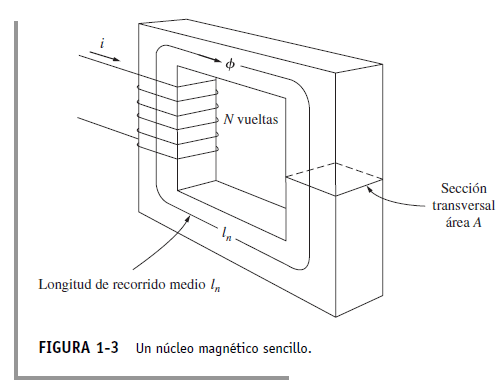
En un núcleo de material ferromagnético como el que se muestra en la Figura 1.3:


La magnitud de la densidad de flujo está dada por:

null

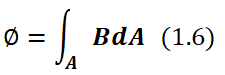
Donde ln es la longitud media del núcleo, y la corriente Ineta que pasa por el camino de integración es igual a Ni, puesto que la bobina de alambre corta dicho camino N veces mientras pasa la corriente i. Ahora, el flujo total Ø en cierta área del núcleo está dado por:

null

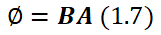
Donde dA es el diferencial del área. Si el vector de densidad de flujo es perpendicular a un plano de área A y si la densidad de flujo es constante en toda el área, la ecuación se reduce a:

null

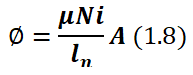
Si sustituimos la ecuación 1.5 en 1.7 obtenemos la ecuación 1.8, una interesante relación que demuestra como la corriente en una bobina de alambre conductor enrollado alrededor de un núcleo de material ferromagnético, produce un flujo magnético en dicho material.

null

Puesto que los motores y generadores dependen del flujo magnético para producir el voltaje y el par, se diseñan para producir el máximo flujo posible. Como resultado, la mayoría de las máquinas reales operan cerca del punto de rodilla de la curva de magnetización.

Fuerza magnetomotriz

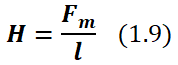
Siempre que existe un flujo magnético Ø en un cuerpo o componente, se debe a la intensidad de un campo magnético H, dada por:

null

Donde Fm es la fuerza magnetomotriz que actúa en el componente (medido en Ampere-vuelta) y l es la longitud del componente (medido en metros).

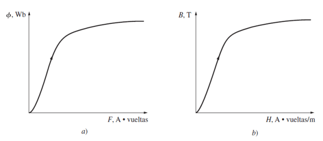
La relación entre el flujo magnético Ø y la fuerza magnetomotriz Fm es semejante aquella que existe entre la densidad de flujo B y la intensidad del campo magnético H, tal como lo ilustra la Figura 1.10.

Es decir, que para un núcleo dado la intensidad del campo magnético es directamente proporcional a la fuerza magnetomotriz, y que la densidad de flujo magnético es directamente proporcional al flujo magnético total.

Curva de Histéresis

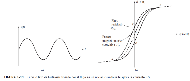
En vez de aplicar una corriente continua a los devanados dispuestos sobre el núcleo, se aplica una corriente alterna para observar qué ocurre. Dicha corriente se muestra en la Figura 1-11 (a). Suponga que el flujo inicial en el núcleo es cero. Cuando se incrementa la corriente por primera vez, el flujo en el núcleo sigue la trayectoria ab, dibujada en la Figura 1-11 (b). Ésta es básicamente la curva de saturación que se muestra en la figura 1-10. Sin embargo, cuando la corriente decrece, el flujo representado en la curva sigue una trayectoria diferente de la seguida cuando la corriente iba en aumento. Cuando la corriente decrece, el flujo en el núcleo sigue la trayectoria bcd y, más tarde, cuando la corriente se incrementa de nuevo, el flujo sigue la trayectoria deb. Nótese que la cantidad de flujo presente en el núcleo depende no sólo de la cantidad de corriente aplicada a los devanados del núcleo, sino también de la historia previa del flujo presente en el núcleo. Esta dependencia de la historia previa del flujo y el seguir una trayectoria diferente en la curva se denomina histéresis. La trayectoria bcdeb descrita en la Figura 1-11 (b), que representa la variación de la corriente aplicada, se denomina curva o lazo de histéresis.

Nótese que si primero se aplica al núcleo una fuerza magnetomotriz intensa y luego se deja de aplicar, la trayectoria del flujo en el núcleo será abc. Cuando se suspende la fuerza magnetomotriz, el flujo no llega a cero, ya que permanece cierto flujo en el núcleo, denominado flujo residual (o flujo remanente), el cual es la causa de los imanes permanentes. Para que el flujo llegue a cero, se debe aplicar al núcleo, en dirección opuesta, cierta fuerza magnetomotriz llamada fuerza magnetomotriz coercitiva.

Circuito Magnético

La relación entre flujo magnético Ø y la fuerza magnetomotriz Fm, da pie a una segunda simplificación de gran valor práctico, el circuito magnético. La ecuación 1.8 nos mostró que una corriente produce un campo magnético. Esto es análogo al voltaje que produce un flujo de corriente en un circuito eléctrico. Es posible entonces definir un circuito magnético cuyo comportamiento esté determinado por ecuaciones análogas a aquellas establecidas para un circuito eléctrico.

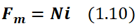
En un circuito eléctrico, el voltaje V genera una corriente I a lo largo de una resistencia R, tal como se ilustra en la Figura 1-4 (a). El voltaje es una fuerza electromotriz que genera el flujo de corriente. Por analogía, en un circuito magnético esta fuerza es Fm de la ecuación 1.9, la cual es igual al flujo efectivo de corriente aplicado al núcleo, es decir:

null

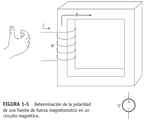
Al igual que la fuente de voltaje, fuerza magnetomotriz Fm tiene una polaridad asociada a ella. Dicha polaridad se determina mediante la regla de la mano derecha, como muestra la Figura 1-5:

null


La fuerza Fm ocasiona un flujo magnético Ø. Si la relación entre el voltaje V y la corriente I en un circuito eléctrico está determinada por V=RI, de forma similar, la relación entre Fm y Ø es:

null

Donde ℜ es la reluctancia del circuito.

Más sobre circuito magnético en la próxima entrega: Circuito Magnético.

Finalizado el Martes 08 noviembre, 2017, 4:57 am

ANTERIOR: Movimiento Rotatorio – Conceptos básicos

SIGUIENTE: Circuito Magnético

Fuentes:

  1. Maquinas Eléctricas-Chapman-5ta-edición
  2. Circuitos magnéticos y transformadores ee staff mit
  3. Analysis of Electric Machinery and Drive Systems
  4. Dynamic simulation of Electric Machinery using MATLAB
  5. Getty Images


Escrito por Prof. Larry Francis Obando – Technical Specialist – Educational Content Writer – Twitter: @dademuch

Se hacen trabajos, ejercicios, clases online, talleres, laboratorios, Academic Paper, Tesis, Monografías….Entrega Inmediata !!!…Comunícate conmigo a través de:

  • WhatsApp: +34 633129287
  • dademuchconnection@gmail.com

Te brindo toda la asesoría que necesites!! …

Mentoring Académico / Emprendedores / Empresarial

Copywriting, Content Marketing, Tesis, Monografías, Paper Académicos, White Papers (Español – Inglés)

Escuela de Ingeniería Electrónica de la Universidad Simón Bolívar, USB Valle de Sartenejas.

Escuela de Ingeniería Eléctrica de la Universidad Central de Venezuela, UCV CCs

Escuela de Turismo de la Universidad Simón Bolívar, Núcleo Litoral.

Contacto: Jaén – España: Tlf. 633129287

Caracas, Quito, Guayaquil, Lima, México, Bogotá, Cochabamba, Santiago.

WhatsApp: +34 633129287

Twitter: @dademuch

FACEBOOK: DademuchConnection

email: dademuchconnection@gmail.com

Electronic Engineer, Power Electronics

Power Electronics – Introduction

Introduction

In broad terms, the task of power electronics is to process and control the flow of electric energy by supplying voltages and currents in a form that is optimally suited for user loads.

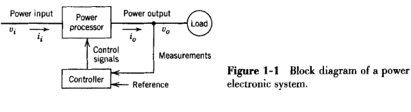
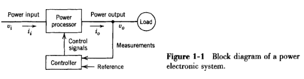
Figure 1-1 shows a power electronic system in a block diagram form. The power input to this power processor is usually (but not always) from the electric utility at a line frequency of 60 or 50 Hz, single phase or three phases. The phase angle between the input voltage and the current depends on the topology and the control of the power processor. The processed output (voltage, current, frequency, and the number of phases) is as desired by the load. If the power processor’s output can be regarded as a voltage source, the output current and the phase angle relationship between the output voltage and the current depend on the load characteristic. Normally, a feedback controller compares the output of the power processor unit with a desired (or a reference) value, and the error between the two is minimized by the controller. The power flow through such systems may be reversible, thus interchanging the roles of the input and the output.

In recent years, the field of power electronics has experienced a large growth due to confluence of several factors. The controller in the block diagram of Fig. 1-1 consists of linear integrated circuits and/or digital signal processors. Revolutionary advances in microelectronics methods have led to the development of such controllers. Moreover, these advances in semiconductor fabrication technology have made it possible to significantly improve the voltage- and current-handling capabilities and the switching speeds of power semiconductor devices, which make up the power processor unit of Fig. 1-1. At the same time, the market for power electronics has significantly expanded. Electric utilities in the United States expect that by the year 2000 over 50% of the electrical load may be supplied through power electronic systems such as in Fig. 1-1.

Power Electronics Defined

It has been said that people do not use electricity, but rather they use communication, light, mechanical work, entertainment, and all the tangible benefits of both energy and electronics. In this sense, electrical engineering is a discipline very much involved in energy conversion and information. In the general world of electronics engineering, the circuits engineers design and use are intended to convert information, with energy merely a secondary consideration in most cases. In radio frequency applications, energy and information are sometimes on a more equal footing, but the main function of any circuit is that of information transfer.

What about the conversion and control of electrical energy itself? Electrical energy sources are varied and of many types. It is natural, then, to consider how electronic circuits and systems can be applied to the challenges of energy conversion and management. This is the framework of power electronics, a discipline that is defined in terms of electrical energy conversion, applications, and electronic devices. More specifically,

DEFINITION: Power electronics involves the study of electronic circuits intended to control the flow of electrical energy. These circuits handle power flow at levels much higher than the individual device ratings.

Power Electronics Vs Linear Electronics

In any power conversion process such as that shown by the block diagram in Fig. 1- 1, a small power loss and hence a high energy efficiency is important because of two reasons: the cost of the wasted energy and the difficulty in removing the heat generated due to dissipated energy.

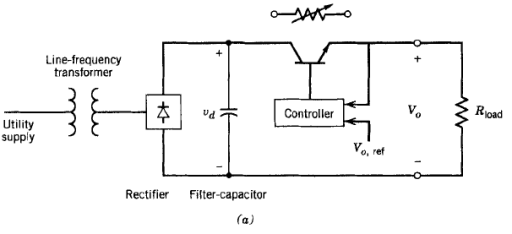
Other important considerations are reduction in size, weight, and cost. The above objectives in most systems cannot be met by linear electronics where the semiconductor devices are operated in their linear (active) region and a line-frequency transformer is used for electrical isolation. As an example, consider the direct current (dc) power supply of Fig. 1-2a to provide a regulated output voltage V, to a load.

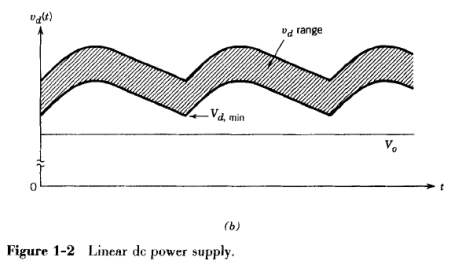
The utility input may be typically at 120 or 240 V and the output voltage may be, for example, 5 V. The output is required to be electrically isolated from the utility input. In the linear power supply, a line-frequency transformer is used to provide electrical isolation and for stepping down the line voltage. The rectifier converts the alternating current (ac) output of the transformer low-voltage winding into dc. The filter capacitor reduces the ripple in the dc voltage vd. Figure 1-2b shows the vd waveform, which depends on the utility voltage magnitude (normally in a t 10% range around its nominal value).

The transformer turns ratio must be chosen such that the minimum of the input voltage v, is greater than the desired output V. For the range of the input voltage waveforms shown in Fig. 1-2b, the transistor is controlled to absorb the voltage difference between v and V, thus providing a regulated output. The transistor operates in its active region as an adjustable resistor, resulting in a low energy efficiency. The line-frequency transformer is relatively large and heavy.

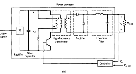
In power electronics, the above voltage regulation and the electrical isolation are achieved, for example, by means of a circuit shown in Fig. 1-3a.

In this system, the utility input is rectified into a dc voltage vd, without a line-frequency transformer. By operating the transistor as a switch (in a switch mode, either fully on or fully 0ff) at some high switching frequency f, for example at 300 kHz, the dc voltage vd is converted into an ac voltage at the switching frequency. This allows a high-frequency transformer to be used for stepping down the voltage and for providing the electrical isolation.

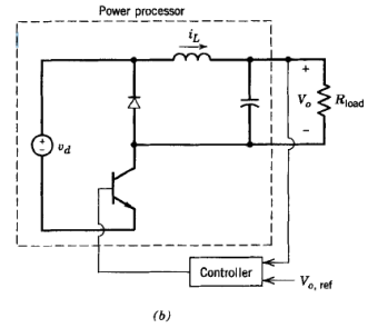
In order to simplify this circuit for analysis, we will begin with the dc voltage vd as the dc input and omit the transformer, resulting in an equivalent circuit shown in Fig. 1-3b.

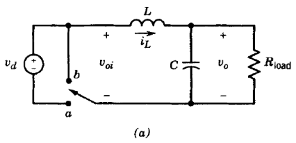
Suffice it to say at this stage that the transistor diode combination can be represented by a hypothetical two-position switch shown in Fig. 1-4a (provided iL(t) > 0).

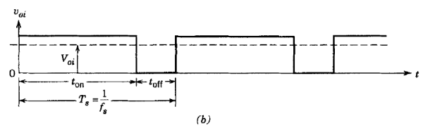
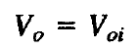
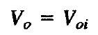
The switch is in position a during the interval t-on, when the transistor is on and in position b when the transistor is off during t-off. As a consequence, Voi equals Vd, and zero during t-on and t-off, respectively, as shown in Fig. 1-4b.

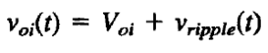
Let us define

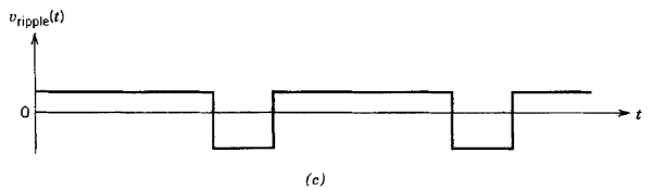
where Voi is the average (dc) value of Voi-t, and the instantaneous ripple voltage V-ripple, which has a zero average value, is shown in Fig. 1-4c.

The L-C elements form a low-pass filter that reduces the ripple in the output voltage and passes the average of the input voltage, so that

where Vo, is the average output voltage. From the repetitive waveforms in Fig. 1-4b, it is easy to see that

As the input voltage Vd changes with time, Eq. 1-3 shows that it is possible to regulate Vo, at its desired value by controlling the ratio t-on/Ts which is called the duty ratio D of the transistor switch. Usually, Ts (= l/fs) is kept constant and t-on is adjusted.

There are several characteristics worth noting. Since the transistor operates as a switch, fully on or fully off, the power loss is minimized. Of course, there is an energy loss each time the transistor switches from one state to the other state through its active region. Therefore, the power loss due to switchings is linearly proportional to the switching frequency. This switching power loss is usually much lower than the power loss in linear regulated power supplies.

At high switching frequencies, the transformer and the filter components are very small in weight and size compared with line-frequency components.

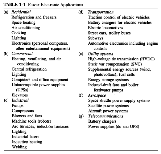
Scope and Applications of Power Electronics 

The expanded market demand for power electronics has been due to several factors discussed below:

  • Switch-mode (dc) power supplies and uninterruptible power supplies. Advances in microelectronics fabrication technology have led to the development of computers, communication equipment, and consumer electronics, all of which require regulated dc power supplies and often uninterruptible power supplies.
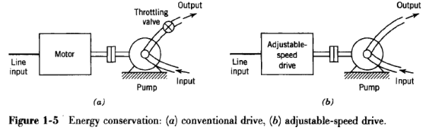
  • Energy conservation. Increasing energy costs and the concern for the environment have combined to make energy conservation a priority. One such application of power electronics is in operating fluorescent lamps at high frequencies (e.g., above 20 kHz) for higher efficiency. Another opportunity for large energy conservation is in motor-driven pump and compressor systems. In a conventional pump system shown in Fig. 1-5a, the pump operates at essentially a constant speed, and the pump flow rate is controlled by adjusting the position of the throttling valve. This procedure results in significant power loss across the valve at reduced flow rates where the power drawn from the utility remains essentially the same as at the full flow rate. This power loss is eliminated in the system of Fig. 1-56, where an adjustable-speed motor drive adjusts the pump speed to a level appropriate to deliver the desired flow rate.

  • Process control and factory automation. There is a growing demand for the enhanced performance offered by adjustable-speed-driven pumps and compressors in process control. Robots in automated factories are powered by electric servo (adjustable-speed and position) drives. It should be noted that the availability of process computers is a significant factor in making process control and factory automation feasible.
  • Transportation. In many countries, electric trains have been in widespread use for a long time. Now, there is also a possibility of using electric vehicles in large metropolitan areas to reduce smog and pollution. Electric vehicles would also require battery chargers that utilize power electronics.
  • Electro-technical applications. These include equipment for welding, electroplating, and induction heating.
  • Utility-related applications. One such application is in transmission of power over high-voltage dc (HVDC) lines. At the sending end of the transmission line, line-frequency voltages and currents are converted into dc. This dc is converted back into the line-frequency ac at the receiving end of the line. Power electronics is also beginning to play a significant role as electric utilities attempt to utilize the existing transmission network to a higher capacity. Potentially, a large application is in the interconnection of photovoltaic and wind-electric systems to the utility grid.
Classification of Power Processors and Converters

For a systematic study of power electronics, it is useful to categorize the power processors, shown in the block diagram of Fig. 1-1, in terms of their input and output form or frequency.

In most power electronic systems, the input is from the electric utility source. Depending on the application, the output to the load may have any of the following forms:

  1. dc
    1. regulated (constant) magnitude
    2. adjustable magnitude
  2. ac
    1. constant frequency, adjustable magnitude
    2. adjustable frequency and adjustable magnitude

The utility and the ac load, independent of each other, may be single phase or three phase. The power flow is generally from the utility input to the output load.

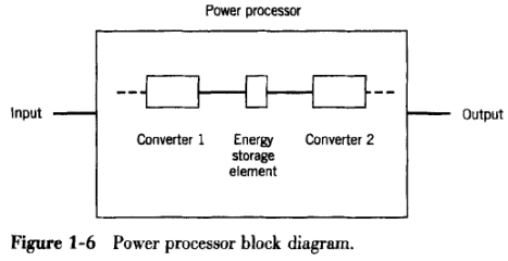
The power processors of Fig. 1-1 usually consist of more than one power conversion stage (as shown in Fig. 1-6) where the operation of these stages is decoupled on an instantaneous basis by means of energy storage elements such as capacitors and inductors.

Therefore, the instantaneous power input does not have to equal the instantaneous power output. We will refer to each power conversion stage as a converter. Thus, a converter is a basic module (building block) of power electronic systems. It utilizes power semiconductor devices controlled by signal electronics (integrated circuits) and possibly energy storage elements such as inductors and capacitors. Based on the form (frequency) on the two sides, converters can be divided into the following broad categories:

  1. ac to dc
  2. dc to ac
  3. dc to dc
  4. ac to ac

We will use converter as a generic term to refer to a single power conversion stage that may perform any of the functions listed above. To be more specific, in ac-to-dc and dc-to-ac conversion, rectifier refers to a converter when the average power flow is from the ac to the dc side. Inverter refers to the converter when the average power flow is from the dc to the ac side.

Further insight can be gained by classifying converters according to how the devices within the converter are switched. There are three possibilities:

  1. Line frequency (naturally cornmutated) converters, where the utility line voltages present at one side of the converter facilitate the turn-off of the power semiconductor devices. Similarly, the devices are turned on, phase locked to the line voltage waveform. Therefore, the devices switch on and off at the line frequency of 50 or 60 Hz.
  2. Switching (forced-commutated) converters, where the controllable switches in the converter are turned on and off at frequencies that are high compared to the line frequency.
  3. Resonant and quasi-resonant converters, where the controllable switches turn on and/or turn off at zero voltage and/or zero current.

Interdisciplinary Nature of Power Electronics

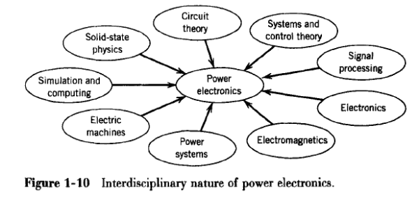
The discussion in this introductory chapter shows that the study of power electronics encompasses many fields within electrical engineering, as illustrated by Fig. 1- 10.

Combining the knowledge of these diverse fields makes the study of power electronics challenging as well as interesting. There are many potential advances in all these fields that will improve the prospects for applying power electronics to new applications.

Sources:

  1. Power Electronic – Mohan
  2. Libro Rashid – Power Electronic Handbook

Literature Review by: Larry Francis Obando – Technical Specialist

Lunes 15 de noviembre, 11:08 am – Caracas, Quito, Guayaquil.

Escuela de Ingeniería Eléctrica de la Universidad Central de Venezuela, Caracas.

Escuela de Ingeniería Electrónica de la Universidad Simón Bolívar, Valle de Sartenejas.

Escuela de Turismo de la Universidad Simón Bolívar, Núcleo Litoral.

Contact: Ecuador (Quito, Guayaquil, Cuenca) telf. +34633129287

WhatsApp: +34633129287

email: dademuchconnection@gmail.com

Internet of Things

Defining IoT Business Models – 1st

Date: October 2017, Location: Caracas, Quito, Guayaquil, Ecuador.

Actividad WBS
Miércoles 04, 5:37 am


I read the report:

  1. Defining IoT Business Models(Canonical)

How to start a business with IoT

1st Literature Review

Post by Canonical:

Highlights

  1. For many businesses looking to take their first step into IoT, how to start and the benefits are unclear issues.
  2. There are three key elements to start with: how can IoT be monetized, what skill are required and addressing fundamental security concerns.

From the connected factories of Siemens and AirBus, through to smart home products of Samsung and Bosch, the Internet of Things is providing businesses with a whole new platform upon which to build innovative products, processes and new business models.

With a current market valuation of over $900bn1, both manufacturers and those looking to adopt IoT solutions are well aware of the potential of IoT. However, in trying to leverage this potential, many business are still grappling with how IoT can benefit their business and the best approach to get started with their IoT initiative.

IoT Dilemma

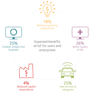
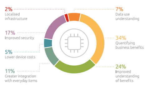
Businesses see massive opportunities in IoT, but are also aware of significant challenges Broadly-speaking, respondents to Canonical’s survey see a number of basic ways in which the internet of things might benefit the business community:

While a quarter of IoT professionals are focused on the opportunities offered by new connected products and services, just as many are excited by the potential big data insights that connected technology could provide their brands.

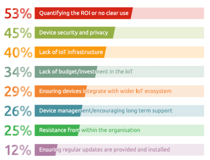
These same professionals stated that the most immediate challenges they are faced by IoT are:

Similarly, when asked what they believed was needed in order to encourage IoT adoption among enterprises, the top priorities to emerge were:

While IoT professionals recognise the potential of IoT, it’s clear that they believe the underlying business case and how to get started implementing IoT needs to be better understood. The above findings indicate not only concerns about security, as to be expected, but also how they set up an IoT ready organisation and how to turn their investment into one that can drive new revenue growth. In addressing these points, this report will answer three simple questions:

1. ‘How can IoT investments be monetised (and justified)?’

2. ‘What skills are needed in order to develop and maximise

IoT solutions?’

3. ‘How can the industry address the issue of IoT security?’

Approaches to monetizing IoT

Many organizations are struggling to understand what many would argue to be the most important question in IoT – how, exactly, will they make a return on their investments? This section will look to explore the different routes to monetization and which may be most wise for the long run.

Many vendor companies will continue to profit through hardware sales

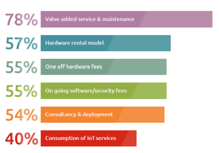
As it stands, 55% of IoT professionals see their profits as coming from the sale of hardware. And with hardware revenues continuing to go up, driven by the sheer volume of hardware required by the IoT, these hardware vendors can be confident of the fact that they will continue to make decent money for some time to come.

With chipsets and electronics dominating the cost of IoT devices, it’s a natural place to explore when trying to determine the future of IoT hardware. With every generation of IoT hardware, we are witnessing an increase in processing ability, a reduction in size, and ultimately, a significant reduction in cost. As electronic hardware becomes cheaper year after year it potentially means lower bills of material and higher margins for hardware vendors.

The reality however is very different. The pressure of commoditization means that without product differentiation, the downward pressure on price is stronger than the reducing cost of the bill of material. This leaves hardware vendors with little choice; either choose more expensive custom components with a price premium and serve less price sensitive, niche markets, or use commoditized components and try to differentiate.

This second approach is the one chosen by an increasing number of IoT device manufacturers, turning their backs on bespoke hardware solutions and choosing instead to fit their devices with fully general-purpose single-board computers (SBCs) or system-onchips (SoCs).

Where once the idea of running a full computer rather than a simple microcontroller would have been viewed as overkill (both in terms of cost and functionality), as the size and price of SBCs such as the Raspberry Pi or Orange Pi has plummeted, developers can now justify using them as a low-cost, high-power alternatives at the heart of all of their IoT devices.

So how are IoT businesses looking to differentiate and turn profit in the Internet of Things?

Monetising IoT – Expected monetization methods of IoT

Profit will be increasingly driven by services and software – which are also potential monetization routes for owner/operators.

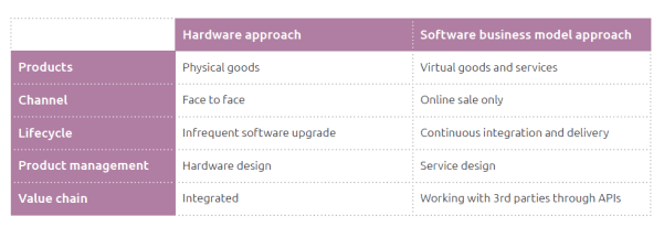
The results from the survey question above speak loud and clear with IoT vendors exploring a number of new business models to complement hardware and envisaging that the sale of software and services promises greater revenues. We can see that the overall percentage of IoT revenue represented by hardware is on the decline. 78% of IoT professionals agree that the real monetization of connected devices will lie in the creation, deployment and maintenance of value-added services, with 40% stating it will be, specifically, through the consumption of services. With the exception of consultancy services, all the other monetization models are from scalable productised services. And the only way to deliver these services is through embedded or cloud software which effectively turns a hardware product into a ‘thing as a service’.

This shifting of the value center sharply towards software is rendered possible only by the commoditized electronics available to hardware vendors. In a world where all compute can affordably be general-purpose, the functionality of virtually all devices will be defined by the software running on them. But this shift of value also needs a change of approach from device manufacturers to put software right at the heart of their product.

This valuable new avenue for monetization can only come from a connected device using a general-purpose-compute SoC/SBC, that treats software, not as a one off component that ships with the hardware and never changes again, but instead as an essential part of the product that will evolve over time and that can be bundled and monetized in a number of ways. This starts with the operating system and extends all the way to the business specific applications being run on the device.

As a result a versatile, IoT specific operating system such as Ubuntu Core, that can be repeatedly upgraded and has the ability to add new functionality in the form of apps plays a key role to opening up the IoT to new based software business models.

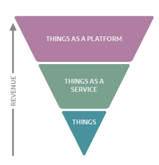
There are a number of additional business models at play in IoT today, including:

Things as a platform

• Revenue from industrial insights: for example, sale of failure analysis stats

gleaned from industrial machinery

• Revenue from personal insights: similar to the above but at a consumer level,

for example, the sale of anonymised fitness tracker data

• Revenue from 3rd parties creating applications for your hardware

Things as a service

• Support: for example, repairs resulting from the prediction that a device will require maintenance could result in the device-owner saving money further down the line. Repairs can also be directly monetized, and can result in improved brand loyalty

• The use of IoT devices for context-specific advertising

• Value from the interaction of human factors and machine interaction: for example, warning a consumer when their device detects it is too close to a source of danger (‘pay per warning”)

The opportunities that these business models present to device manufacturers are much more attractive than the old hardware opportunities. However, migrating to these approaches requires a mindset shift from hardware manufacturers:

This is a paradigm shift not dissimilar to the one the consumer software industry went through when migrating from shrinkwrapped software to app store business models.

Profiting through IoT app stores

An ‘app store for things’ is the natural extension of the app store concept. But rather than being applied to software applications running on a phone they apply to any new software-based service that can be offered on a ‘thing’.

App stores for things have the following characteristics:

• They can be used to distribute any type of software-based service: new functionalities, reconfigurations, analytics and so on

• They offer an online sales channel

• They take care of the software distribution without any effort from the developer

• They can be used to distribute securely any software, whether internal or 3rd party

• They can be ‘white labelled’ to offer services specific to the device they are installed on

Through the development of an IoT app store, businesses can offer add-ons and enhancements to their existing connected devices, charging users to download and install packaged applications to build upon their existing IoT technology. Such stores represent an opportunity not only for vendors, but also for software vendors and system integrators to widen the market for their software and services.

This software sales or app store approach is set to fundamentally change the way that businesses benefit from investments in the internet of things, with 55% of IoT professionals saying that they intend to monetize their devices through the use of ongoing software-led upgrades.

The ‘app store for things’ can be used in a variety of ways. For example, Lime Microsystem, producers of mobile base stations, use a white label appstore from Canonical to let base station owners configure their device in one click and turn a 4G base station into e.g. a powerful Wi-Fi hotspot. Lime Microsystem uses the fact that the configuration file that makes the hardware a 4G base station or a Wi-Fi hotspot is only a piece of software, and packages that configuration file as an application that can be downloaded from a store.

It is also worth bearing in mind that, while the term ‘app store’ is usually associated with paid third party applications, it is also possible for companies to use an app store as a simple yet effective distribution mechanism to distribute their own software – either as a means of delivering upgrades or to patch devices en masse in-the-field.

In a world where every connected device generates data, the opportunities for monetizing this data are limited only by your access and your imagination. We’re likely to see a number of until now unpredicted methods of monetization emerge as the industry develops further.

It is this approach that Canonical promotes through its growing work in the IoT space, encouraging the adoption of a single IoT operating system6 upon which advancements and new functionalities can easily be developed and delivered via snaps.

This is the future of the IoT – a future of software defined everything. But in the same way that companies require new approaches to software distribution to approach the IoT they also need a new set of talents.

Identifying and hiring the right skills

Of course, there’s little point choosing a business model or technology unless you have the capabilities necessary to deliver on them. Many businesses are concerned by their own lack of knowledge and skills within the IoT market. With high potential for profit and low barriers to entry, widespread promotion of the internet of things has led many technology brands into a gold rush of IoT investment and product design. Unfortunately, given its relatively new status, many business leaders have found themselves running headfirst into a set of technology and business challenges that they do not yet fully understand. What they need is a new generation of talent with the knowledge and skills to navigate the current Wild West that is the internet of things.

The evolving architecture in the IoT landscape is rapidly moving from basic end-point devices delivering data to cloud applications to a more diverse and complex computing model. This means that in addition to the need for data science and security skills, that are in short supply, distributed computing skills are also emerging as an important requirement. Any current ‘full stack’ developer or architect now has to be aware of many more components, it may be anything from machine learning, Artificial Intelligence or Blockchain to new user interfaces such as Augmented Reality or communication stacks on emerging networking protocols. The physical world presents design challenges too, where time of day, remote locations or weather conditions can alter the ability to operate reliably.

The first question that an organisation looking to embrace IoT needs to address is what skills they require and whether any of these already exist in-house. The sheer scale and scope of IoT means there is a plethora of skills that could be required depending on the project or projects within an organisation. The requirements for these may vary and evolve over time, meaning that organisations need teams who are multi-functional and thus generalists by nature but also cover a number of specialisms across the entire software stack from low level embedded code to machine learning capabilities in the cloud. Inevitably some of these skills will be commonplace already but IoT will also increase the need for skills that weren’t previously required.

It’s not just cloud development talents that are required. When asked what skills they deemed necessary to be an IoT expert, after data analytics (at 75%) software development skills were found to be the most needed skill (according to 71% of IoT professionals). In one sense this is surprising, as embedded development is by no means a new discipline. But when considering the fact that hardware is rapidly commoditizing, with monetization and differentiation increasingly coming from software, it is natural that businesses invest in building up their embedded software development capabilities. Unfortunately, 33% are struggling to hire employees with this particular skillset.

Full article: Defining IoT Business Models

Review by: Larry Francis Obando – Technical Specialist

Escuela de Ingeniería Eléctrica de la Universidad Central de Venezuela, Caracas.

Escuela de Ingeniería Electrónica de la Universidad Simón Bolívar, Valle de Sartenejas.

Escuela de Turismo de la Universidad Simón Bolívar, Núcleo Litoral.

Contact: Ecuador (Caracas, Quito, Guayaquil, Cuenca)

WhatsApp: 00593984950376

email: dademuchconnection@gmail.com
Copywriting, Content Marketing, Tesis, Monografías, Paper Académicos, White Papers (Español – Inglés)

Circuit Analysis, Ecuaciones Diferenciales, Electrical Engineer, Elementos Básicos, Literature Review, Señales y Sistemas, Sin categoría

EL CAPACITOR. Relación corriente-voltaje.

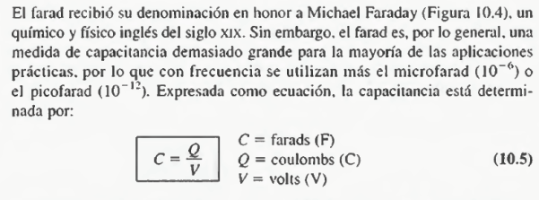
Formalmente, la Capacitancia es la razón entre la carga de una placa del capacitor y la diferencia de tensión entre las dos placas:

null

Relación corriente-voltaje del capacitor

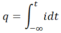
Para obtener la relación de corriente-tensión del capacitor, primero es necesario estudiar la relación entre la carga q y la corriente i. Dicha relación viene dada por la ecuación:

null

Para encontrar la carga q de las placas en el tiempo t se integra sobre todo el tiempo anterior:

null

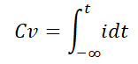
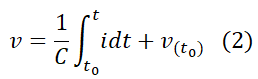
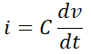
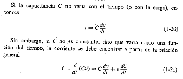
Utilizando el hecho de que q=Cv, obtenemos la relación corriente-tensión del capacitor (suponiendo un capacitor lineal, es decir, que no depende del valor de la tensión v en el tiempo):

null

null

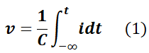
O sea:

null

Otra forma de presentar este resultado es mediante la fórmula:

null

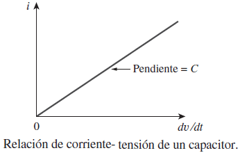
Utilizando esta última ecuación, podemos graficar la relación corriente-voltaje del capacitor de la manera siguiente:

null

Recomiendo leer la siguiente guía: Capacitores e Inductores – Circuitos y asociaciones

Preliminares

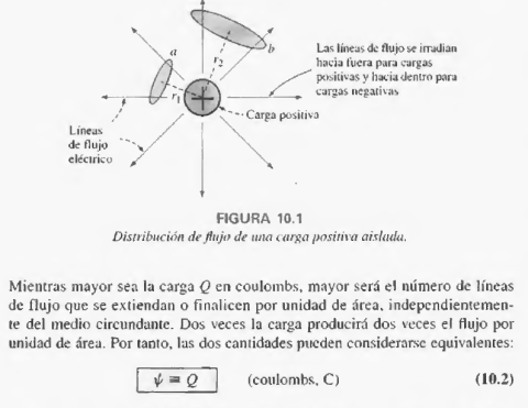
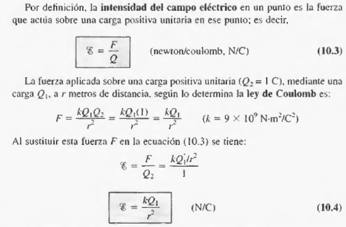
Por tanto se concluye que la intensidad del campo eléctrico en cualquier punto a una distancia r de una carga puntual de Q coulombs, será directamente proporcional a la magnitud de la carga e inversamente proporcional al cuadrado de la distancia a la carga.

Capacitancia

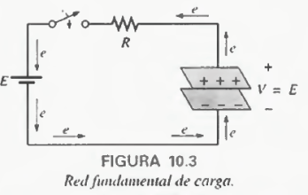
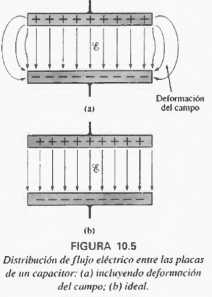
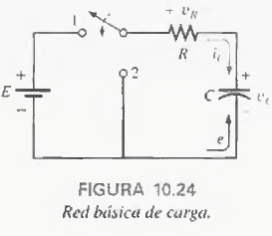
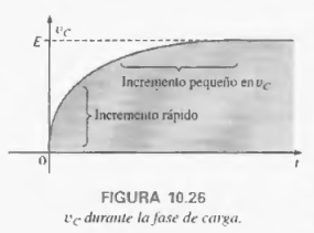
Al instante en que el interruptor se cierra, se extraen los electrones de la placa superior y se depositan sobre la placa inferior debido a la batería, dando por resultado una carga neta positiva sobre la placa superior del capacitor y una carga negativa sobre la placa inferior…Cuando el voltaje en el capacitor es igual al de la batería, cesa la transferencia de electrones y la placa tendrá una carga neta Q=CV=CE

En este punto el capacitor asumirá las características de un circuito abierto: una caída de voltaje en las placas sin flujo de carga entre las placas.

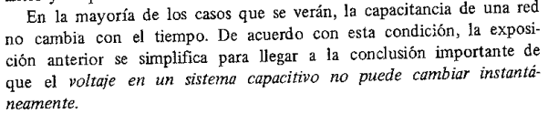
El voltaje en un capacitor no puede cambiar de forma instantánea.

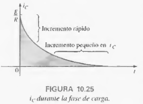
De hecho, la capacitancia en una red es también una medida de cuanto se opondrá ésta a un cambio en el voltaje de la red. Mientras mayor sea la capacitancia, mayor será la constante de tiempo y mayor el tiempo que le tomará cargar hasta su valor final

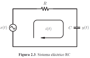
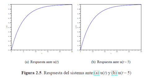
Ejemplo 2.2 (Fuente:3) La Figura 2.3 muestra un sistema compuesto por una resistencia y un capacitor, y cuyos valores son representados respectivamente por R y C. Además, la figura muestra que el sistema eléctrico es excitado por una señal x(t) = u(t) y su respuesta es medida a través de la tensión sobre el capacitor, donde u(t) representa la función escalón unitario:

El modelo matemático asociado al sistema representado por la Figura 2.3 puede obtenerse empleando elementales ecuación de redes eléctricas:

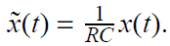
Entonces, al comparar el modelo matemático definido por la Ecuación (2.12) con el modelo obtenido, se tiene que el coeficiente a0 y la señal de excitación son:

,

Al aplicar la solución expresada por medio de la Ecuación (2.21), se puede afirmar que:

Al operar la Ecuación (2.26) se tiene que la respuesta del sistema es dada por:

Note que:

por cuanto el elemento de memoria representado por el capacitor no permite cambios bruscos y por tal motivo y(0-) = y(0) = y(0+). Además, para buscar una respuesta a la pregunta debe tomarse en cuenta que la excitación tiene un valor de cero y ella ha permanecido en cero desde mucho tiempo atrás, es decir, desde menos infinito, obviamente y(0) = 0.

Recomiendo leer la siguiente guía: Capacitores e Inductores – Circuitos y asociaciones

Fuentes:

  1. Introduccion-al-analisis-de-circuitos-robert-l-boylestad,
    1. El Parámetro Capacitancia p 20
  2. Análisis de Redes – Van Valkenburg,
    1. El Parámetro Capacitancia p 20
  3. Análisis de Sistemas Lineales – Prof. Ebert Brea
    1. Análisis de Sistemas en el Dominio Continuo pp 29 –
  4. Fundamentos_de_circuitos_electricos_5ta

SIGUIENTE:

Escrito por Prof. Larry Francis Obando – Technical Specialist – Educational Content Writer – Twitter: @dademuch

Se hacen ejercicios, problemas, trabajos, clases online…Respuesta inmediata !!! a través de: WhatsApp: +34 633129287

Mentoring Académico / Emprendedores / Empresarial

Copywriting, Content Marketing, Tesis, Monografías, Paper Académicos, White Papers (Español – Inglés)

Escuela de Ingeniería Electrónica de la Universidad Simón Bolívar, USB Valle de Sartenejas.

Escuela de Ingeniería Eléctrica de la Universidad Central de Venezuela, UCV CCs

Escuela de Turismo de la Universidad Simón Bolívar, Núcleo Litoral.

Contacto: Jaén – España: Tlf. 633129287

Caracas, Valladolid, Quito, Guayaquil, Jaén, Ordizia, Zaragoza.

WhatsApp: +34 633129287

Twitter: @dademuch

FACEBOOK: DademuchConnection

email: dademuchconnection@gmail.com
Computer Science, UML

UML – Requirements Elicitation

The client, the developers, and the users identify a problem area and define a system that addresses the problem. Such a definition is called a requirements specification and serves as a contract between the client and the developers…The requirements specification is structured and formalized during analysis to produce an analysis model…(August 7, 2017).

The first step of requirements elicitation is the identification of actors. This serves both to define the boundaries of the system and to find all the perspectives from which the developers need to consider the system…(September 18, 2017).

Actividad WBS (Overview)
Fuente:

  1. Object-Oriented Software Engineering
    1. Requirement Elicitation concepts – Functional requirements
    2. Requirement Elicitation activities -Identifying actors – Identifying scenarios – Identifying Use Cases – Identifying relationships between actors and Use Cases – Identifying Initial Analysis Objects -Identifying Non-functional requirements – Documenting Requirements Elicitation- (p 152).
A requirement is a feature that the system must have or a constraint that it must satisfy to be accepted by the client. Requirements engineering aims at defining the requirements of the system under construction. Requirements engineering includes two main activities; Requirements Elicitation, which results in the specification of the system that the client understands, and analysis, which results in an analysis model that the developers can unambiguously interpret. Requirements elicitation is the more challenging of the two because it requires the collaboration of several groups of participants with different backgrounds. On the one hand, the client and the users are experts in their domain and have a general idea of what the system should do, but they often have little experience in software development. On the other hand, the developers have experience in building systems, but often have little knowledge of the everyday environment of the users.

Requirement elicitation

Overview

A requirement is a feature that the system must have or a constraint that it must satisfy to be accepted by the client. Requirements engineering aims at defining the requirements of the system under construction. Requirements engineering includes two main activities; Requirements Elicitation, which results in the specification of the system that the client understands, and analysis, which results in an analysis model that the developers can unambiguously interpret. Requirements elicitation is the more challenging of the two because it requires the collaboration of several groups of participants with different backgrounds. On the one hand, the client and the users are experts in their domain and have a general idea of what the system should do, but they often have little experience in software development. On the other hand, the developers have experience in building systems, but often have little knowledge of the everyday environment of the users.

Scenarios and use cases provide tools for bridging this gap. A scenario describes an example of system use in terms of a series of interactions between the user and the system. A use case is an abstraction that describes a class of scenarios. Both scenarios and use cases are written in natural language, a form that is understandable to the user. In this chapter, we focus on scenario-based requirements elicitation.,,Requirements elicitation is about communication among developers, clients, and users to define a new system…Requirements elicitation methods aim at improving communication among developers, clients, and users…Developers construct a model of the application domain by observing users in their environment. Developers select a representation that is understandable by the clients and users (e.g., scenarios and use cases). Developers validate the application domain model by constructing simple prototypes of the user interface and collecting feedback from potential users…Requirements elicitation focuses on describing the purpose of the system. The client, the developers, and the users identify a problem area and define a system that addresses the problem. Such a definition is called a requirements specification and serves as a contract between the client and the developers…The requirements specification is structured and formalized during analysis to produce an analysis model:

Both requirements specification and analysis model represent the same information. They differ only in the language and notation they use; the requirements specification is written in natural language, whereas the analysis model is usually expressed in a formal or semiformal notation.

Requirements elicitation and analysis focus only on the user’s view of the system. For example, the system functionality, the interaction between the user and the system, the errors that the system can detect and handle, and the environmental conditions in which the system functions are part of the requirements. The system structure, the implementation technology selected to build the system, the system design, the development methodology, and other aspects not directly visible to the user are not part of the requirements.

Requirements elicitation includes the following activities:

  1. Identifying actors
  2. Identifying scenarios
  3. Identifying use cases
  4. Refining use cases
  5. Identifying relationships among use cases
  6. Identifying nonfunctional requirements

Elicitation concepts

Functional requirements describe the interactions between the system and its environment independent of its implementation. The environment includes the user and any other external system with which the system interacts… The functional requirements focus only on the possible interactions between the system and its external world. This description does not focus on any of the implementation details.

Nonfunctional requirements describe aspects of the system that are not directly related to the functional behavior of the system. Nonfunctional requirements include a broad variety of requirements that apply to many different aspects of the system, from usability to performance. The FURPS+ model2 used by the Unified Process [Jacobson et al., 1999] provides the following categories of nonfunctional requirements:

Elicitation Activities

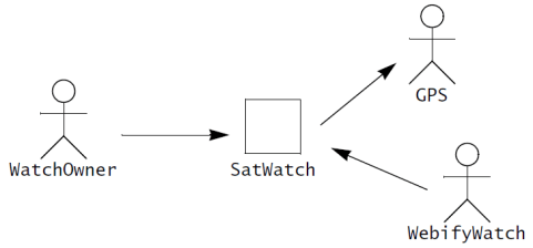
Identifying Actors: Actors represent external entities that interact with the system. An actor can be human or an external system. In the SatWatch example, the watch owner, the GPS satellites, and the Webify Watch serial device are actors (see Figure 4-4). They all exchange information with the SatWatch.

Figure 4-4 Actors for the SatWatch system. WatchOwner moves the watch (possibly across time zones) and consults it to know what time it is. SatWatch interacts with GPS to compute its position. Webify Watch upgrades the data contained in the watch to reflect changes in time policy.

The first step of requirements elicitation is the identification of actors. This serves both to define the boundaries of the system and to find all the perspectives from which the developers need to consider the system. When the system is deployed into an existing organization (such as a company), most actors usually exist before the system is developed: they correspond to roles in the organization. During the initial stages of actor identification, it is hard to distinguish actors from objects. For example, a database subsystem can at times be an actor, while in other cases it can be part of the system. Note that once the system boundary is defined, there is no trouble distinguishing between actors and such system components as objects or subsystems. Actors are outside of the system boundary; they are external. Subsystems and objects are inside the system boundary; they are internal.

Thus, any external software system using the system to be developed is an actor. When identifying actors, developers can ask the following questions:

Questions for identifying actors:

• Which user groups are supported by the system to perform their work?

• Which user groups execute the system’s main functions?

• Which user groups perform secondary functions, such as maintenance and administration?

• With what external hardware or software system will the system interact?

Identifying Scenarios: A scenario is “a narrative description of what people do and experience as they try to make use of computer systems and applications” [Carroll, 1995]. A scenario is a concrete, focused, informal description of a single feature of the system from the viewpoint of a single actor. Scenarios cannot (and are not intended to) replace use cases, as they focus on specific instances and concrete events (as opposed to complete and general descriptions). However, scenarios enhance requirements elicitation by providing a tool that is understandable to users and clients…

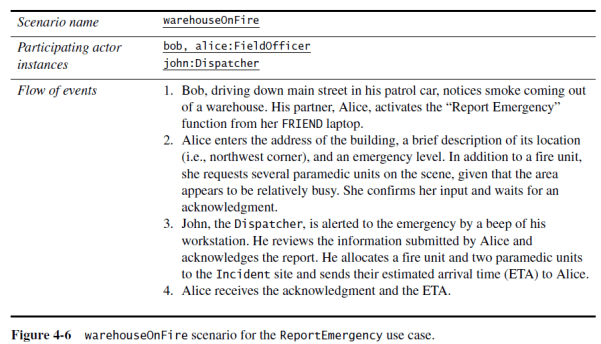
Figure 4-6 is an example of scenario for the FRIEND system, an information system for incident response. In this scenario, a police officer reports a fire and a Dispatcher initiates the incident response.

Scenarios can have many different uses during requirements elicitation and during other activities of the life cycle. Below is a selected number of scenario types taken from [Carroll, 1995]:

As-is scenarios describe a current situation. During reengineering, for example, the current system is understood by observing users and describing their actions as scenarios.

Visionary scenarios describe a future system. Visionary scenarios are used both as a point in the modeling space by developers as they refine their ideas of the future system and as a communication medium to elicit requirements from users.

Evaluation scenarios describe user tasks against which the system is to be evaluated. The collaborative development of evaluation scenarios by users and developers also improves the definition of the functionality tested by these scenarios.

Training scenarios are tutorials used for introducing new users to the system. These are step-by-step instructions designed to hand-hold the user through common tasks.

In requirements elicitation, developers and users write and refine a series of scenarios in order to gain a shared understanding of what the system should be. Initially, each scenario may be high level and incomplete, as the warehouseOnFire scenario is. The following questions can be used for identifying scenarios.

Questions for identifying scenarios

• What are the tasks that the actor wants the system to perform?

• What information does the actor access? Who creates that data? Can it be modified or removed? By

whom?

• Which external changes does the actor need to inform the system about? How often? When?

• Which events does the system need to inform the actor about? With what latency?

Identifying Use Cases: A scenario is an instance of a use case; that is, a use case specifies all possible scenarios for a given piece of functionality. A use case is initiated by an actor. After its initiation, a use case may interact with other actors, as well. A use case represents a complete flow of events through the system in the sense that it describes a series of related interactions that result from its initiation…Figure 4-7 depicts the use case ReportEmergency of which the scenario warehouseOnFire (see Figure 4-6) is an instance

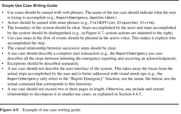
Generalizing scenarios and identifying the high-level use cases that the system must support enables developers to define the scope of the system. Initially, developers name use cases, attach them to the initiating actors, and provide a high-level description of the use case as in Figure 4-7. The name of a use case should be a verb phrase denoting what the actor is trying to accomplish. The verb phrase “Report Emergency” indicates that an actor is attempting to report an emergency to the system (and hence, to the Dispatcher actor). This use case is not called “Record Emergency” because the name should reflect the perspective of the actor, not the system. It is also not called “Attempt to Report an Emergency” because the name should reflect the goal of the use case, not the actual activity

Attaching use cases to initiating actors enables developers to clarify the roles of the different users. Often, by focusing on who initiates each use case, developers identify new actors that have been previously overlooked.

Describing the flow of events of a use case enables developers and clients to discuss the interaction between actors and system. This results in many decisions about the boundary of the system, that is, about deciding which actions are accomplished by the actor and which actions are accomplished by the system.

Identifying relationships between actors and Use Cases: Communication relationships between actors and use cases represent the flow of information during the use case. The actor who initiates the use case should be distinguished from the other actors with whom the use case communicates. By specifying which actor can invoke a specific use case, we also implicitly specify which actors cannot invoke the use case. Similarly, by specifying which actors communicate with a specific use case, we specify which actors can access specific information and which cannot. Thus, by documenting initiation and communication relationships among actors and use cases, we specify access control for the system at a coarse level.

Identifying Initial Analysis Objects: To establish a clear terminology, developers identify the participating objects for each use case. Developers should identify, name, and describe them unambiguously and collate them into a glossary.3 Building this glossary constitutes the first step toward analysis, which we discuss in the next chapter. The glossary is included in the requirements specification and, later, in the user manuals. Developers keep the glossary up to date as the requirements specification evolves. The benefits of the glossary are manyfold: new developers are exposed to a consistent set of definitions, a single term is used for each concept (instead of a developer term and a user term), and each term has a precise and clear official meaning. The identification of participating objects results in the initial analysis object model. The identification of participating objects during requirements elicitation only constitutes a first step toward the complete analysis object model.

During requirements elicitation, participating objects are generated for each use case. If two use cases refer to the same concept, the corresponding object should be the same. If two objects share the same name and do not correspond to the same concept, one or both concepts are renamed to acknowledge and emphasize their difference. This consolidation eliminates any ambiguity in the terminology used.

Identifying Non-functional requirements: Nonfunctional requirements describe aspects of the system that are not directly related to its functional behavior. Nonfunctional requirements span a number of issues, from user interface look and feel to response time requirements to security issues. Nonfunctional requirements are defined at the same time as functional requirements because they have as much impact on the development and cost of the system.

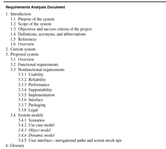
Documenting Requirements Elicitation: The results of the requirements elicitation and the analysis activities are documented in the Requirements Analysis Document (RAD). This document completely describes the system in terms of functional and nonfunctional requirements.Figure 4-16 is an example template for a RAD:

Written by: Larry Francis Obando – Technical Specialist

Escuela de Ingeniería Eléctrica de la Universidad Central de Venezuela, Caracas.

Escuela de Ingeniería Electrónica de la Universidad Simón Bolívar, Valle de Sartenejas.

Escuela de Turismo de la Universidad Simón Bolívar, Núcleo Litoral.

Contact: Caracas, Valladolid, Quito, Guayaquil, Jaén, Villafranca de Ordizia – +34633129287

WhatsApp: +34633129287

email: dademuchconnection@gmail.com

Copywriting, Content Marketing, Tesis, Monografías, Paper Académicos, White Papers (Español – Inglés)

Ecuaciones Diferenciales, Matemática aplicada - Appd Math

Introduction to differential equation and modeling

Fuente: Introduction to Differential Equations

    1. Motivation
    2. A secret function
    3. Cell division
    4. Classification of differential equations
    5. Homogeneous linear ODE
    6. Introduction to modeling
    7. Model of a savings account
    8. Application: mixing salt water solution
    9. Systems and signals
    10. Newtonian mechanics
    11. 5 step modeling process

Today’s objectives

  1. Identify linear first order differential equations.
  2. Model behavior of certain systems using first order linear differential equations.
  3. Use the input signal and system response paradigm to obtain an ODE for a physical system.
  4. Check reasonableness of models using unit analysis .


Definition 3.2 An initial value problem is a differential equation together with initial conditions.


4. Cell division

Here we will see how the differential equation for our secret function appears when modeling a natural phenomenon – the population growth of a colony of cells…In this example we’ll model the number of yeast cells in a batch of dough. As we work through this example, pay careful attention to the assumptions we make, and how the initial condition plays a role in the resulting differential equation.

For our system, we assume we have a colony of yeast cells in a batch of bread dough. The first step is to identify the variables, the units, and give them names.

y

number of cells

t

time measured in seconds

We also need to set some initial condition, y0, the number of cells that we begin with at t=0. In this system, this might be the number of yeast cells in a yeast packet.

A differential model

If y denotes the number of yeast cells, what can we say about the derivative y˙? The derivative represents the rate at which the number of cells is growing. How should it depend on the number of cells? In nature, cells given plenty of space and food tend to divide through mitosis regularly. If we assume that each cell is dividing independently of all other cells, then doubling the number of cells should double the rate at which new cells are born. In fact, multiplying the number of cells by any scalar factor should do the same to the derivative. So this directly implies that the growth rate of cells is proportional to the number of cells:

y˙∝y.

We can make this into a true equation by simply inserting a proportionality constant a, such that

y˙=ay.

We say that 1/a is a “characteristic» timescale for our problem, setting the rate at which the cells divide. A solution to the above differential equation is

where y0 is the number of yeast cells we started with at t=0. In our case, we assume that y0 is the number of yeast cells in a packet, which is about 180 billion yeast cells.

5. Classification of differential equations

Marcar esta página

There are two kinds:

  • An ordinary differential equation (ODE) involves derivatives of a function of only one variable.
  • A partial differential equation (PDE) involves partial derivatives of a multivariable function.

When we consider ODEs, we will often regard the independent variable to be time…The dot notation y˙ should only be used to refer to a time derivative. If for example y is a function of a spacial variable y=y(x), we will only use the notation y′ to denote the derivative with respect to x.

Definition 5.1 The order of a DE is the highest n such that the nth derivative of the function appears…

The order is 5, because the highest derivative that appears is the 5th derivative, y(5).

7. Natural growth and decay equations..We’ve been introduced to a few basic forms of differential equations so far. The first equation we saw was a basic growth equation,

y˙=ay,

which, when a is a positive constant, governs systems like bank accounts and cell populations. If we put a negative sign in front of a we get the decay equation

y˙=−ay,

which can be used to describe things like radioactive decay of materials.

How would you classify the differential equations y˙=ay and y˙=−ay just discussed? Choose all descriptors that apply…
Solution:

These two equations are both first order, linear, homogeneous differential equations. To see that these equations are homogeneous, we can either check that y=0 is a solution (it is), or we can rewrite them in standard linear form:

8. Introduction to modeling

Marcar esta página

There are two kinds of modeling. We’re not going to talk about the kind that involves fancy clothes and photographs. The other kind, mathematical modeling , is converting a real-world problem into mathematical equations.

Guidelines:

  1. Identify relevant quantities, both known and unknown, and give them symbols. Find the units for each.
  2. Identify the independent variable(s). The other quantities will be functions of them, or constants. Often time is the only independent variable.
  3. Write down equations expressing how the functions change in response to small changes in the independent variable(s). Also write down any “laws of nature» relating the variables. As a check, make sure that all summands in an equation have the same units.

Often simplifying assumptions need to be made; the challenge is to simplify the equations so that they can be solved but so that they still describe the real-world system well.

I have a savings account earning interest compounded daily, and I make frequent deposits or withdrawals into the account. Find an ODE with initial condition to model the balance.

Simplifying assumptions:

  • Daily compounding is almost the same as continuous compounding, so let’s assume that interest is paid continuously instead of at the end of each day.
  • Similarly, let’s assume that my deposits/withdrawals are frequent enough that they can be approximated by a continuous money flow at a certain rate, the net deposit rate (which is negative when I am withdrawing).

Variables and functions (with units): Define the following:

P

the initial amount that the account starts with (dollars)

t

time from the start (years)

x

balance (dollars)

I

the interest rate (year−1; for example 4%/year=0.04year−1)

q

the net deposit rate (dollars/year).

Here t is the independent variable, P is a constant, and x, I, q are functions of t.

Equations: Now we want to decide how the balance changes as time changes. We’ll estimate the change in the balance Δxas time increases from some time t to a time t+Δt. We can approximate the interest earned per dollar to be:

Note that the units in each of the three terms are dollars/year. Also, there is the initial condition x(0)=P. Thus we have an ODE with initial condition:

Now that the modeling is done, the next step might be to solve this DE, but we won’t do that yet.

Remark 9.2 The notation we chose suggested that the interest rate I depended only on time. However, I could have depended on x as well. This would not change the modeling process. If I does not depend on x, we obtain a linear differential equation. If it does, the equation is nonlinear.

Video: Application: mixing salt water solution

Systems and signals

Let’s get back to the savings account model:

x˙=I(t)x+q(t).

Maybe for financial planning I am interested in testing different saving strategies (different functions q) to see what balances x they result in. To help with this, rewrite the ODE as

In the “systems and signals» language of engineering, q is called the input signal , the bank is the system , and x is the output signal . These terms do not have a mathematical meaning dictated by the DE alone; their interpretation is guided by the system being modeled. But the general picture is this:

The system may be a mechanical system such as an automobile suspension or an electrical circuit, or an economic market. It is impacted by some external signal. We are interested in understanding how the system responds to the external stimulus.

  • The input signal is the external stimulus. It usually does not appear in as simple a way in the DE as it does in the example above. But it does always determine the right hand side of the DE (when written in standard linear form).
  • The system response (also called output signal ) is the measurable behavior of the system that we are interested in. It is always the unknown function that we write a differential equation for.
  • All differential equations have many solutions. The solution of interest is often determined by the state of the system at the beginning. This initial state is given by the initial conditions.

Newtonian mechanics

Let’s try to put this into the input/ system response paradigm we’ve just introduced. The system response is the displacement of the mass. This is what we are interested in.

What is the input signal? You could imagine that there are other forces acting on the mass, like there is a sail on the mass, and wind is blowing on the sail creating an input signal. But we are going to start by considering the case where the input signal is 0. Note that pulling the cart back and releasing it specifies the initial state of the system, that is, it gives the initial conditions.

Now we are ready to write down the differential equation . The equation is governed by Newton’s second law

We need to identify the forces acting on the mass. There is the force due to the spring. For the moment, we assume that air resistance is negligible, and there is no friction on the cart.

What is the spring force? When the displacement is positive, the spring is stretched, the force is negative. When the displacement is negative, the spring is compressed, the force is positive. Thus this force is modeled linearly by Hooke’s law:

which is a function of the displacement x away from the neutral position x=0. Note that this linear model is only valid for relatively small displacements. If we stretch the spring too far, the spring force won’t obey this linear law anymore.

The position at time t=0 is x(0)=x0 for some positive displacement x0>0. From the problem statement, we assume that we release the cart with zero initial velocity, x˙(0)=0.

Putting this all together, we get:

with initial conditions:

The last step is to write this in standard linear form . We obtain the following differential equation:

Now let’s consider the same mass/spring system as above where we’ve add a sail to the mass.

The mass now experiences an additional external force from the wind. How does this change the model?

Solution: The model is exactly the same. The only difference is that the input signal is no longer zero, rather it is now the external force due to the wind on the sail. This external force Fwind(t) depends on time in some complicated way that we will not try to write down. The differential equation for this system is:

5 step modeling process

Marcar esta página

In the example on the previous page, we outlined a 5 step modeling process that we make explicit here.

  1. Draw a diagram of the system.
  2. Identify and give symbols for the parameters and variables of the system.
  3. Decide on the input signal and the system response. Identify any initial conditions.
  4. Write down a differential equation relating the input signal and the system response.
  5. Rewrite the equation in standard linear form with initial conditions.

Written by: Larry Francis Obando – Technical Specialist

Escuela de Ingeniería Eléctrica de la Universidad Central de Venezuela, Caracas.

Escuela de Ingeniería Electrónica de la Universidad Simón Bolívar, Valle de Sartenejas.

Escuela de Turismo de la Universidad Simón Bolívar, Núcleo Litoral.

Contact: Ecuador (Quito, Guayaquil, Cuenca)

WhatsApp: 00593984950376

email: dademuchconnection@gmail.com
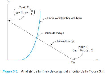
Copywriting, Content Marketing, Tesis, Monografías, Paper Académicos, White Papers (Español – Inglés)

Matemática aplicada - Appd Math, Señales y Sistemas

Señales de tiempo continuo – Definición

Una señal x(t) es una función con valor real o escalar de la variable de tiempo t. El término con valor real significa que para cualquier valor fijo de la variable de tiempo t, el valor de la señal en el tiempo t es un número real. Cuando esta variable toma sus valores del conjunto de los números reales, se dice que t es una variable de tiempo continuo, y que la señal x(t) es una señal de tiempo continuo o una señal analógica. Ejemplos comunes de señales de tiempo continuo son el voltaje u ondas de corriente de un circuito eléctrico, las señales de audio como voz u ondas musicales, las posiciones o velocidades de objetos en movimiento, las fuerzas o torcas en un sistema mecánico, las señales bioeléctricas como electrocardiogramas (ECG) o electroencefalogramas (EEG), las velocidades de flujo de líquidos o gases en un proceso químico, etc. 

Dada una señal x(t) muy complicada, no siempre es posible determinar una función matemática que sea exactamente igual a x(t). Un ejemplo es una señal de voz, como el segmento de diálogo de 50 milisegundos que aparece en la Figura 1. Este segmento es la transición de la «sh» a «u» de la elocución de la palabra inglesa «should». 

Primero que nada el analista de sistemas debe conocer cómo modelar señales en el dominio del tiempo continuo.

  1. Introducción
  2. Función Escalón
  3. Función Rampa
  4. Función Impulso
  5. Función Pulso Rectangular
  6. Función Pulso Triangular
  7. Función Periódica
  8. Función Exponencial
Función Escalón

Fuente: [3]


Función Rampa


Función Impulso


Función Pulso Rectangular


Función Pulso triangular

Fuente: [2]


Función Periódica

Fuente: [1]

Fuente: [3]

Fuente: [1]


Función Exponencial


Fuente:

Fundamentos_de_Señales_y_Sistemas_usando la Web y Matlab

1.1 Señales en tiempo continuo

SIGUIENTE: Señales de tiempo discreto – Muestreo en matlab.

Written by: Larry Francis Obando – Technical Specialist – Educational Content Creation – Mentoring (Tutoría para estudiantes universitarios)

Escuela de Ingeniería Electrónica de la Universidad Simón Bolívar, Valle de Sartenejas.

Escuela de Ingeniería Eléctrica de la Universidad Central de Venezuela, Caracas.

Escuela de Turismo de la Universidad Simón Bolívar, Núcleo Litoral.

Contact: Caracas, Valladolid, Quito, Guayaquil, Jaén, Villafranca de Ordizia

WhatsApp: +34633129287

email: dademuchconnection@gmail.com
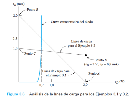
 

Linear Algebra, Matemática aplicada - Appd Math

Linear Algebra – Foundations

Linear Algebra

Start Line:

  1. DLM
    1. Appd Mathematics
      1. Linear Algebra…What You Will Learn:
        • Represent quantities that have a magnitude and a direction as vectors.
        • • Read, write, and interpret vector notations.
        • • Visualize vectors in R2.
        • • Perform the vector operations of scaling, addition, dot (inner) product.
        • • Reason and develop arguments about properties of vectors and operations defined on them.
        • • Compute the (Euclidean) length of a vector.
        • • Express the length of a vector in terms of the dot product of that vector with itself.
        • • Evaluate a vector function.
        • • Solve simple problems that can be represented with vectors.
        • • Create code for various vector operations and determine their cost functions in terms of the size of the vectors.
        • • Gain an awareness of how linear algebra software evolved over time and how our programming assignments fit into this
        • (enrichment).
        • • Become aware of overflow and underflow in computer arithmetic (enrichment).
        • Become practical with the use of Matlab to apply all these framework


PAGE_BREAK: PageBreak

Date: August, September 2017. Location: Quito, Pichincha, Ecuador.

Actividad WBS (Vector Algebra – )
Martes 15, 06:32 am

Martes 29, 04:41 am

Jueves 31, 04:41 am

Lunes 04, 5:37 am

Lunes 11, 5:37 am

Martes 12, 4:46 am

Jueves 14, 5:15 am

I keep attending:

  1. LAFF: Linear Algebra – Foundations to Frontiers
    1. Overview of the Course
    2. 0.3.3 MATLAB Basics
    3. Origins of MATLAB
    4. Vectors in Linear Algebra
      1. Notation
      2. Unit Basis Vectors
      3. Simple Vector Operations
        1. Equality, Assignment and Copy
        2. Vector Addition
        3. Scaling
        4. Subtraction
      4. Advanced Vector Operations
        1. Scaled Vector Addition (AXPY)
        2. Linear Combinations of Vectors
        3. Dot or Inner Product (DOT)
        4. Vector Length (NORM2)
        5. Vector Functions
        6. Vector Functions that map a vector to a vector
    5. The Science of NFL Football: Vectors


This course is not only designed to teach the standard topics in a typical linear algebra course, but it also investigates how to translate theory into algorithms. Like typical in the algebra courses, we will often start studying operations with small matrices. In practice, however, one often wants to perform operations with large matrices so we generalize the techniques to formulate practical algorithms and their implementations
If you want to learn more about MATLAB, here are some suggestions you may want to investigate:

  • Matlab Onramp is a free 2-hour interactive online tutorial.
  • MATLAB Central is a place where people interested in MATLAB can be part of a community. Here, you may want to check out ThingSpeak™, the open loT Platform with MATLAB Analytics that allows you to aggregate, visualize, and analyze live data streams in the cloud.


Definition from Vectors in Linear Algebra

Definition 1.1 We will call a one-dimensional array of n numbers a vector of size n:

denotes the set of all vectors of size n with components in R.

Unit Basis Vectors


Equality, Assignment and Copy


Now we could talk about an algorithm for setting y equal to x. We’re computing y becomes x. We’ve already seen that each of the components of y has to be set to a corresponding component of x. So psi sub i has to become chi sub i. We have to do this for all indices i from 0 to n minus 1. We start indexing at 0, and therefore, if the vectors are of length n, we have to run this until n minus 1. We create an algorithm for this assignment by now writing this as a FOR LOOP.


Vector Addition

Now if we wanted an algorithm for computing the result vector, z, that results from adding x to y, then we can expose the components of z, the components of x and y, and we recognize that the ith of z just equals to the some of the ith components of x and y. And we can then summarise that as a little loop that says for all components of z, for i from 0 to n minus 1, the ith component of z, zeta sub i, should just be computed as chi sub i, added to psi sub i.

Scaling


What if instead we want an algorithm that computes vector y as the stretched vector x stretched by a scaling factor alpha? y becomes alpha times x. We expose the components of y. We need to compute alpha times x, where here we expose the individual components of x. And all we need to do is set the appropriate element of y to the corresponding element of x scaled by alpha. If we do this as an algorithm, then what we need to do to set psi i equal to alpha times chi i.

Subtraction


Let’s review the parallelogram method for vector addition. You lay out your vectors as such. And then, the diagonal becomes x:

You can do the same thing for vector subtraction. You lay out your vectors. And then, the other diagonal becomes the vector x minus y. Obviously, you have to make sure that it points in the right direction.

Now, how do you compute x minus y? Well, you expose the different components of vectors x and y. And you simply subtract each component of y off the corresponding component of x.

In Summary:

Scaled Vector Addition (AXPY)


We’re now going to talk about an operation that is going to be very important as we start looking at more complex operations, and then the algebra later on. It’s hard to picture though. It’s known as the axpy operation, and it takes a vector, scales it, and then adds it to another vector. Given two vectors x and y of size n and a scalar alpha, the axpy operation is given by y is equal to alpha x plus y.

Specifically


These kinds of vector operations have been very important since the 1970s, and back then the language of choice in this area was Fortran 77. Fortran 77 had the limitation that the variables and subroutines had to be identified with at most six letters and numbers. So they had to be somewhat innovative about how to name operations, and subroutines that implemented them. And the axpy here is simply an abbreviation of alpha times x plus y. So it stands for scalar alpha, the a, times x, plus, p, y–axpy.


If we now want to look at an algorithm for performing this operation, notice that the i-th component of y has to be updated by scaling the i-th component of x and adding it to the i-th component of y. So psi i becomes alpha times chi i plus psi i. And as usual, we need to put a loop around that so this is done for all components zero to n minus 1.

About the AXPY operation, it is often emphasized that it is typically used in situations where the output vector overwrites the input vector y.

Linear Combinations of Vectors

If we’re given two vectors of length m, u and v, and two scalars, alpha and beta, then taking the linear combination of u and v with coefficients alpha and beta is given by alpha times u plus beta times v. So that’s the scalar times the vector u, plus the scalar times the vector v. If we expose the components of u and v, then what does this mean? It means that we scale the first vector, that mean scale each of the individual components, by alpha. And we scale the components of vector v by beta. And that gives us, this right here. So taking this linear combination of vectors u and v, using the coefficients alpha and beta, means that we take the same linear combination of each of the components of u and v.

More generally

Well, instead of writing things like this, we could write them like this. What is that? That’s an AXPY. Why? 0 is a vector. And then this is a scalar times a vector, which you add to that vector. Once you’ve computed this vector, you take a scalar times the second vector and add it to that. So now, the first AXPY, we computed this. The second AXPY computes this. And you can imagine that we can do that for all of the vectors until we’re completely done.

This then motivates the following algorithm. You start by setting w equal to 0. And then for j equals 0 to n minus 1, you perform this operation right here where you take a the scalar chi j times v j and at that to w. So for j equals 0, that’s this operation. That then is stored in w. Then this here is what you do for j equals 1 and so forth.

Shortly, this will become really important as we make the connection between linear combinations of vectors, linear transformations, and matrices.

Dot or Inner Product (DOT)


If we’re given vectors x and y of size n, then the dot product is defined as follows.

Now what do we have here? We multiply the first components together, and then we multiply the second components together, and add those to the first components. And then we keep doing that until we get to the last components. We multiply those together, and we add those in as well. We can write this more concisely as I equals 0 to n minus one, of Chi i times Psi i.

Now to motivate an algorithm, let’s look at this slightly differently. Let’s think of this as, take an alpha, and first assigning 0 to it. After that, we multiply the first two components together, and we add that to 0. After that, we multiply the next two components together, and we add that to what already is in alpha, and so forth…This motivates the algorithm given here. You start by setting alpha equal to zero. And then, for i equals zero to n minus 1, you take what is already accumulated in alpha, and you add to it the product of the components Chi i and Psi i.

Now often we will use a slightly different notation to denote the dot product. OK, the dot product is given by this. We will often write this as x transpose y. OK? This T here means transposition. Now what does transposition mean? If we expose the components of x and y, then the transposition means that you take x, which is a column vector, and you make it into a row vector, as such. So the column vector turns into a row vector. Transposition means taking the vector and putting it on its side. And then multiplying the row vector times a column vector means multiplying the first components together, and adding that to the second components multiplied together, and so forth.

Vector Length (NORM2)

If we take that further and we look at a vector of size n, then the length of that vector is given by the square root of the squares of the components,which we can use shorthand to write as the sum of the squares of the components.

There’s a relation between the dot product and the length of a vector.

And therefore, we conclude that the length of vector x is just a square root of the dot products of x with itself. We summarize that right here.

Vector Function


A vector function is a function that takes one or more scalars and/or one or more vectors as inputs and then produces a vector as an output.

Well, let’s look an an example. So here we have an example of f, which is a function of two scalars. How do we know these are scalars? Well, notice that I’m using Greek letters. We agree that the Greek lowercase letters we were going to use for scalars. So it takes two scalars as input, alpha and beta, and then produces a vector of size two as output, where the first component adds the two input scalars and the second component subtracts the second scalar from the first scalar.

If we want to evaluate f of -2, 1, then all we do is we substitute -2 in for alpha. And we substitute 1 in for beta. So this here then would be the vector -2 plus 1, -2, minus 1. And if you do the arithmetic, you get the vector -1, -3. That’s summarized right here.

Let’s do another example. Here we have a function of the scalar and a vector of size three. And the output is that vector, except that each of its components has been changed by adding the scalar to it. So if you want to evaluate this function for a specific input, -2 for the scalar and the vector 1, 2, 3, then again what we need to do is substitute the -2 in for alpha. And we need to substitute 1, 2, and 3 in for the components of the vector that’s the input.

We have seen other examples already. We saw the AXPY operation, which if you think of it as a function, is the function axpy of a scalar alpha and then vectors x and y. And the output is the vector alpha times x plus y. We also saw the DOT function. And notice that in the DOT function, you have two vectors as input, x and y. And the result is the DOT product of the two factors, which is a scalar. Now you might say a scalar is not a vector. But we’re going to think of a scalar often as a vector of size one.

What we will see in the next unit is that we can think of these vector functions as mapping one vector to another vector.

Vector Functions that map a vector to a vector

Now we’re ready to look at functions that map vectors to vectors. Next week, we’ll look at a special case of those kinds of functions called «linear transformations.» We’re going to be looking at our functions that map a vector of size n to a vector of size m.

In the previous units, we looked at a function that took two scalars as input and produced a vector as an output.

We can look at a function g that takes as input a vector with components alpha and beta and then produces the exact same vector as the function f produced.

Here was another example of a function that took as input a scalar and a vector.

We can instead look at a function g, but now stacks scalar on top of the vector creating a vector that is of size four instead of the size three vector that we had before and then evaluates in exactly the same way.

The whole point being that now we have a function that takes as input a vector and as output, produces a vector.

So in summary, this insight allows us to focus on vector functions that simply take one vector as input and produce one vector as output. What we will see next week is that there’s a special class of such functions called «linear transformations» that are of great importance to linear algebra.

Written by: Larry Francis Obando – Technical Specialist

Escuela de Ingeniería Eléctrica de la Universidad Central de Venezuela, Caracas.

Escuela de Ingeniería Electrónica de la Universidad Simón Bolívar, Valle de Sartenejas.

Escuela de Turismo de la Universidad Simón Bolívar, Núcleo Litoral.

Contact: Ecuador (Quito, Guayaquil, Cuenca)

WhatsApp: 00593984950376

email: dademuchconnection@gmail.com
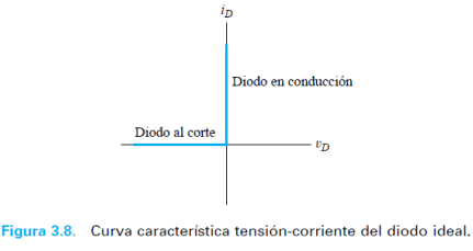
Copywriting, Content Marketing, Tesis, Monografías, Paper Académicos, White Papers (Español – Inglés)