Control System Analysis, PID Control

PID – Basic Control System Actions

BEFORE:  Steady-State error control system

NEXT: PID – Effect of integrative and derivative control actions.

Introduction

An automatic controller compares the real value of the output of a plant with the input reference (the desired value), determines the deviation and produces a control signal that will reduce the deviation to zero or a small value. The way in which the automatic controller produces the control signal is called control action.

Classification of industrial controls

According to their control actions, industrial controllers are classified as:

  1. Two-position (On / Off)
  2. Proportional
  3. Integrals
  4. Proportional-Integrals
  5. Proportional-Derivatives
  6. Proportional-Integrals-Derivatives

Almost all industrial controllers use electricity as an energy source or a pressurized fluid, such as oil or air. The controllers can also be classified, according to the type of energy they use in their operation, like pneumatic, hydraulic or electronic. The type of controller that is used must be decided based on the nature of the plant and operational conditions, including considerations such as safety, cost, availability, reliability, precision, weight and size.

Figure 5-1 shows a typical configuration for an Industrial Control System:
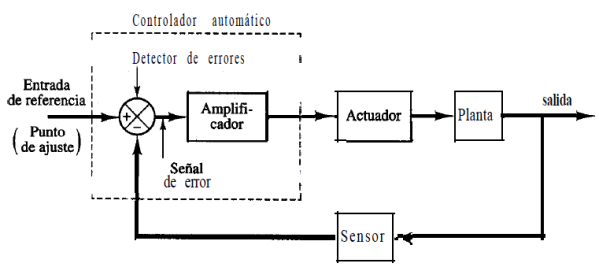
The previous figure consists of a Block Diagram for an industrial control system composed of an automatic controller, an actuator, a plant and a sensor (measuring element). The controller detects the error signal, which is usually at a very low power level, and amplifies it to a sufficiently high level. The output of an automatic controller feeds an actuator that can be a pneumatic valve or an electric motor. The actuator is a power device that produces the input for The plant according to the control signal, so that the output signal approaches the reference input signal. The sensor, or measurement element, is a device that converts an output variable, such as a displacement, into another manageable variable, such as a voltage, that can be used to compare the output with the reference input signal. This element is in the feedback path of the closed-loop system. The setpoint of the controller must be converted into a reference input with the same units as the feedback signal from the sensor or from the measuring element.

Two positions control (On / Off).

In a two position control system, the acting element only has two fixed positions that, in many cases, are simply turned on and off. The On/Off control is relatively simple and cheap, which is why it is extensively used in industrial and domestic control systems.

Suppose that the output signal of the controller is u(t) and that the error signal is e(t). In the control of two positions, the signal u(t) remains at a value either maximum or minimum, depending on whether the error signal is positive or negative. In this way,
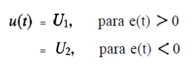
where U1 y U2 are constants. Very often, the minimum value of U2 is zero or –U1.

It is common for two-position controllers to be electrical devices, in which case an electrical valve operated by solenoids is widely used. Pneumatic proportional controllers with very high gains function as two-position controllers and are sometimes referred to as two-position pneumatic controllers.

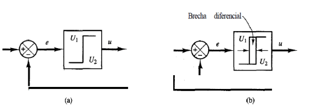
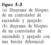
Figures 5-3 (a) and (b) show the block diagrams for two controllers of two positions The range in which the error signal must move before the commutation is called differential gap. In Figure 5-3 (b) a differential gap is indicated. Such a gap causes the output of the controller u (t) to retain its present value until the error signal has moved slightly beyond zero. In some cases, the differential gap is the result of unintentional friction and a lost movement; however, it is often intentionally caused to avoid too frequent operation of the on and off mechanism.
Proportional control action.

For a controller with proportional control action, the relationship between the controller output u (t) and the error signal e (t) is:
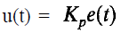
or, in quantities transformed by the Laplace method:
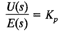
where Kp is considered proportional gain.

Whatever the actual mechanism and the form of the operating power, the controller

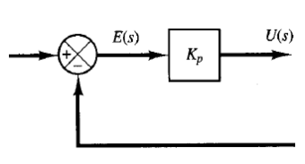
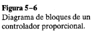
proportional is, in essence, an amplifier with an adjustable gain. A block diagram of such a controller is presented in Figure 5-6.
Integral control action.

In a controller with integral control action, the value of the controller output u (t) is changed to a ratio proportional to the error signal e (t). That is to say,
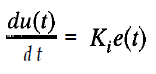
O well:
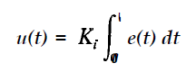
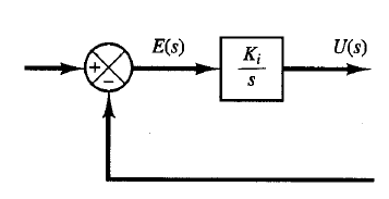
where Ki is an adjustable constant. The transfer function of the integral controller is:
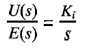
If the value of e (t) is doubled, the value of u (t) varies twice as fast. For an error of zero, the value of u (t) remains stationary. Sometimes, the integral control action is called adjustment control (reset). Figure 5-7 shows a block diagram of such controller.
 

Integral-proportional control action.
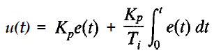
The control action of a proportional-integral controller (PI) is defined by:
null

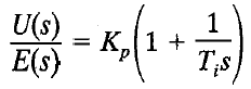
or the transfer function of the controller, which is:
null

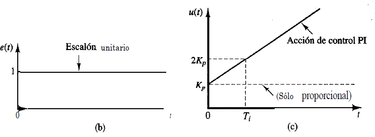
where Kp is the proportional gain and Ti is called integral time. Both Kp and Ti are adjustable. Integral time adjusts the integral control action, while a change in the value of Kp affects the integral and proportional parts of the control action.

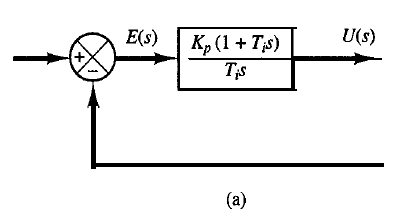
The inverse of the integral time Ti is called the readjustment speed. The rate of readjustment is the number of times per minute that the proportional part of the control action is doubled. The rate of readjustment is measured in terms of the repetitions per minute. The Figure 5-8 (a) shows a block diagram of a PI controller. If the error signal e (t) is a unit step function, as shown in Figure 5-8 (b), the controller output u (t) becomes what is shown in Figure 5-8 (c).
null

null

null

Proportional-derivative control action.
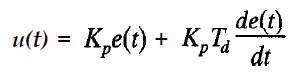
The control action of a proportional-derivative (PD) controller is defined by:
null

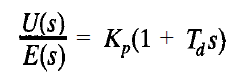
The transfer function is:

null

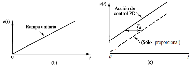
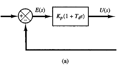
where Kp is the proportional gain and Td is a constant called derivative time. Both Kp and Td are adjustable. The derivative control action, sometimes called speed control, occurs where the magnitude of the controller output is proportional to the rate of change of the error signal. The derivative time Td is the time interval during which the action of the velocity advances the effect of the proportional control action.

Figure 5-9 (a) shows a block diagram of a PD controller. If the error signal e (t) is a unit ramp function as shown in Figure 5-9 (b), the controller output u (t) becomes that shown in Figure 5-9 (c). ). The derivative control action has a forecast nature. However, it is obvious that a derivative control action never foresees an action that has never occurred.null
null

null

Although the derivative control action has the advantage of being forecast, it has the disadvantages that it amplifies the noise signals and can cause a saturation effect in the actuator. Note that the derivative control action is never used alone, because it is only effective during transient periods.

Proportional-Integral-derivative (PID) control action.

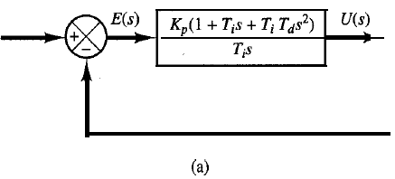
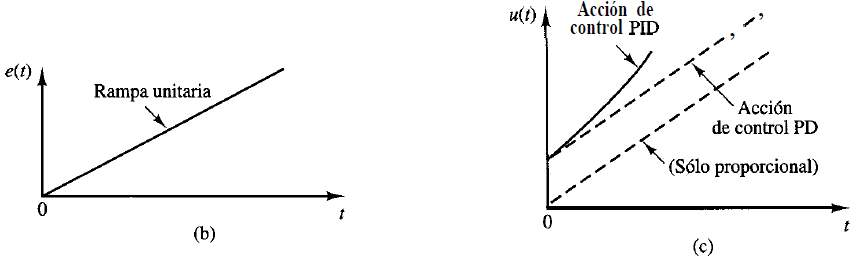
The combination of a proportional control action, an integral control action and a derivative control action is called proportional-integral-derivative (PID) control action.

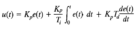
This combined action has the advantages of each of the three individual control actions. The equation of a controller with this combined action is obtained by:
null

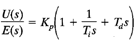
The transfer function is:

null

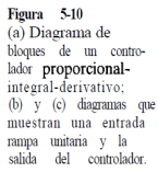
where Kp is the proportional gain, Ti is the integral time and Td is the derivative time. The block diagram of a PID controller appears in Figure 5-10 (a). If e (t) is a unit ramp function, like the one shown in Fig. 5-10 (b), the controller output u (t) becomes that of Fig. 5-10 (c).
null

nullnull

Effects of the sensor on the performance of the system.

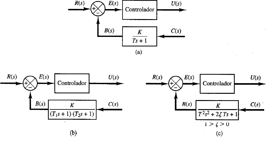
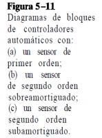
Since the dynamic and static characteristics of the sensor or measuring element affects the indication of the actual value of the output variable, the sensor fulfills a function important to determine the overall performance of the control system. As usual, the sensor determines the transfer function in the feedback path. If the time constants of a sensor are negligible compared to other constants of time of the control system, the sensor transfer function simply it becomes a constant. Figures 5-11 (a), (b) and (c) show diagrams of automatic controller blocks with a first-order sensor, an overdamped second-order sensor and a second-order underdamped sensor, respectively. Often the response of a thermal sensor is of the overdamped second order type.
null

null

BEFORE:  Steady-State error control system

NEXT: PID – Effect of integrative and derivative control actions.

Source:

  1. Ingenieria de Control Moderna, 3° ED. – Katsuhiko Ogata pp 211-232

Literature review by Larry Francis Obando – Technical Specialist – Educational Content Writer

Copywriting, Content Marketing, Tesis, Monografías, Paper Académicos, White Papers (Español – Inglés)

Escuela de Ingeniería Eléctrica de la Universidad Central de Venezuela, CCs.

Escuela de Ingeniería Electrónica de la Universidad Simón Bolívar, Valle de Sartenejas.

Escuela de Turismo de la Universidad Simón Bolívar, Núcleo Litoral.

Contact: Caracas, Quito, Guayaquil, Cuenca. telf – 0998524011

WhatsApp: +593984950376

email: dademuchconnection@gmail.com
Control System Analysis, Time Domain

Transient-response Specifications – Control Systems

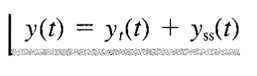
The response in time of a control system is usually divided into two parts: the transient response and the steady-state response. Let y (t) be the response of a system in continuous time, then:

where yt (t) is the transient response, while yss (t) is the steady state response.

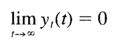
The transient response of a control system is important since both its amplitude and its duration must be kept within tolerable or prescribed limits. It is defined as the part of the response in time that tends to zero when the time becomes very large. Thus,

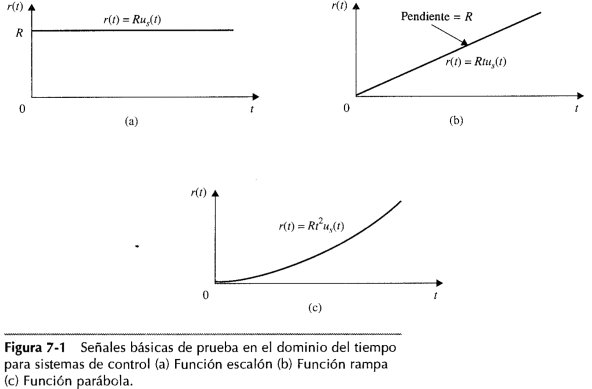
All real stable control systems present a transient phenomenon before reaching the steady state response. For analysis and design purposes it is necessary to assume some basic types of test inputs to evaluate the performance of a system. The proper selection of these test signals allows the prediction of system performance with other more complex inputs. The following signals are used: Step function, which represents an instantaneous change in the reference input; Ramp function, which represents a linear change over time; Parabolic function, which represents a faster order than the ramp. These signals have the common characteristic that they are simple to write in mathematical form, it is rarely necessary or feasible to use faster functions. In Figure 7-1 you can see these functions:

[2]

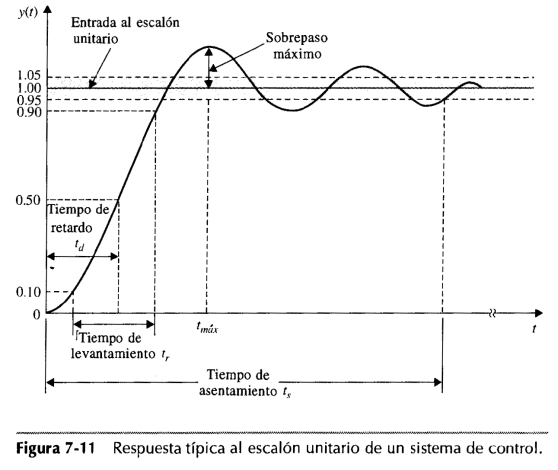
For a linear control system, the analysis and characterization of the transient response is performed frequently using the unit step function Us (t), shown in Figure 7-1a with R = 1. A typical response of a control system to a unit step input is shown in Figure 7-11:

[2]

The transient response of a practical control system often exhibits damped oscillations before reaching the steady state. That’s happens because systems have energy storage and cannot responds immediately. The transient-response to a unit step input depends on the initial conditions. That’s why it is a common practice to use the standard initial conditions that the system is at rest initially with the output an all time derivatives thereof zero.

Second-order systems and Transient-response specifications.

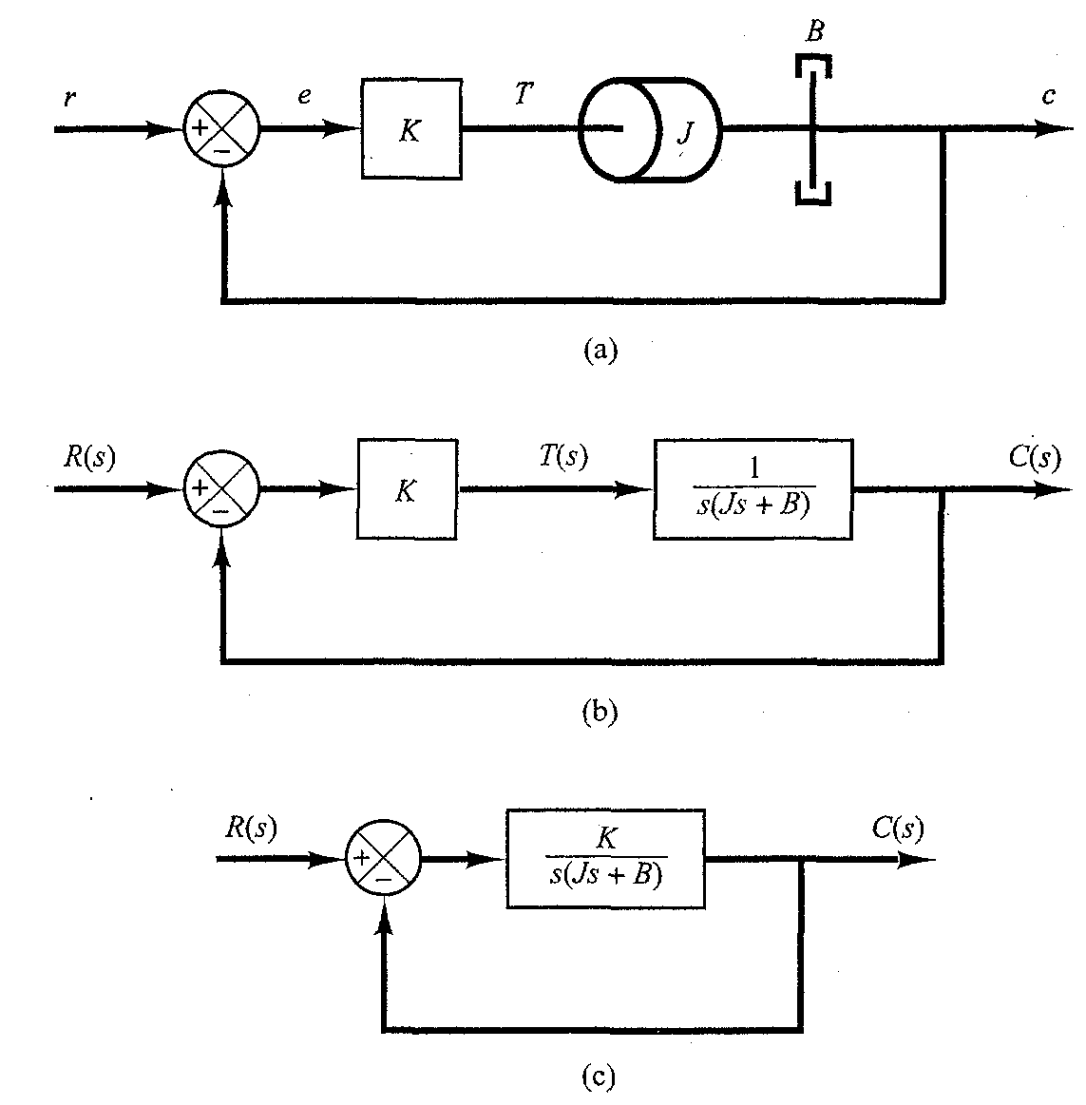
Figure 5-5a shows a Servo System as an example of a second-order system. It consists of a proportional controller and load elements (inertia and viscous friction elements):

null

[3]

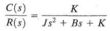
The closed-loop Transfer Function of the system shown in Figure 5-5c is:

In the transient-response analysis it is convenient to write:

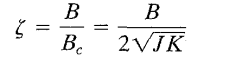
Where σ is called the attenuation; ωn is the undamped natural frequency; and ζ  the damping ratio of the system.  ζ  is the ratio of the actual damping B to the critical damping Bc equal to two times the square-root of JK:

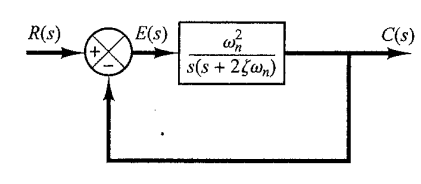
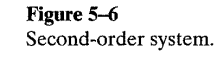
In terms of ωn y σ, the system shown in Figure 5-5c can be expressed as Figure 5-6:

[3]

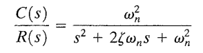
Now, the Transfer Function C(s)/R(s) can be written as:

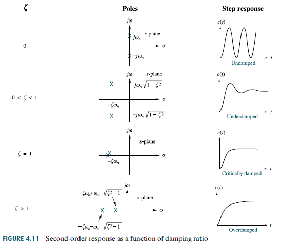
This form is called The Standard Form. The dynamic behavior of a second-order system can be now described in terms of the two parameters ωn and σ. In short, the cases of second-order response as a function of σ are summarized in Figure 4.11 (for a better review see FIRST and SECOND ORDER SYSTEMS):

[1]

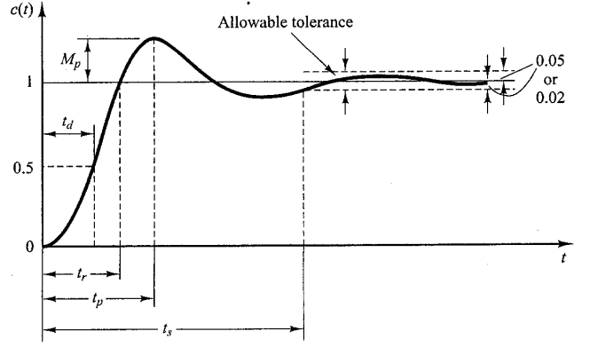
In specifying the transient-response characteristics of a control system to a unit-step input, it is common to specify the following parameters associated with the underdamped response:

  1. Delay time, Td
  2. Rise time, Tr
  3. Peak time, Tp
  4. Percent overshoot (%OS) or Maximum overshoot (Mp)
  5. Settling time, Ts

These specifications are defined as follows:

Delay time (Td): it is the time required for the response to reach half the final value the very first time.

Rise time (Tr): it is the time required for the response to rise from 10% to 90%. In other words, to go from 0.1 of the final value to 0.9 of the final value.

Peak time (Tp): it is the time required for the response to reach the first peak of the overshoot.

Maximum overshoot (Mp): it is the maximum peak value of the response curve measured from unity. It is also the amount that the waveform overshoots the final value, expressed as a percentage of the steady-state value.

Settling time (Ts):  it is the time required for the transient damping oscillations to reach and stay within ±2% or ±5% of the final or steady-state value.

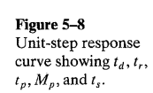
These specifications are graphically shown in Figure 5-8:

[3]

It is important to remark that these specifications don’t necessarily apply to any given case. For example, the terms peak time and maximum overshoot do not apply to overdamped systems.

Except for certain applications where oscillations can’t be tolerated, it is desirable that the transient-response be sufficiently fast and sufficiently damped. Thus, for a desirable transient response of a second-order system, the damping ratio must be between 0.4 and 0.8. Small values of σ (σ<0.4) yields excessive overshoot in the transient response, and systems with a large value of σ (σ>0.8) responds sluggishly. We will also see that the maximum overshoot and the rise time conflict with each other. In other words, they cannot be made smaller simultaneously.

Analytically:
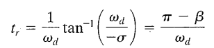
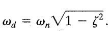
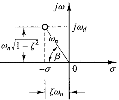
Rise time (Tr):

where ωd is the damped natural frequency:

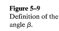
and ß is defined by the Figure 5-9:

[3]

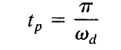
Peak time (Tp):

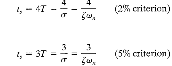
Settling time (Ts):

Transient-response of Higher-order systems.

It could be seen that the transient response of a system higher than a second-order is the sum of the responses of first-order and second order systems.  

Transient-response of a First-order system.

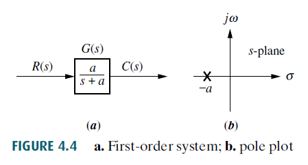
We briefly discuss the transient response of a first-order system. A first-order system without zeros can be described by the transfer function shown in Figure 4.4(a).

[1]

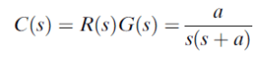
If the input is a unit step, where R(s)=1/s, the Laplace transform of the step response is C(s), where:

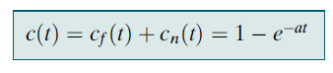
Taking the inverse transform:

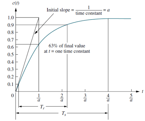
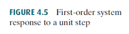
Figure 4-5 shows a typical response of this system to a unit step input:

[1]

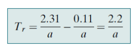
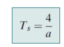
We call 1/a the time constant of the response. The parameter a is the only one needed to describe the transient response for a first-order system. Thus, the time constant can be considered a transient response specification for a first order system, since it is related to the speed at which the system responds to a step input. Since the pole of the transfer function is at a, we can say the pole is located at the reciprocal of the time constant, and the farther the pole from the imaginary axis, the faster the transient response.

The other specifications for a first-order system are:

Rise time (Tr):

Settling time (Ts):

NEXT: Control System Stability

Source:

  1. Control Systems Engineering, Nise pp 177-181
  2. Sistemas de Control Automatico Benjamin C Kuo p 385,
  3. Modern_Control_Engineering, Ogata 4t pp 224, 232

Written by: Larry Francis Obando – Technical Specialist – Educational Content Writer.

Escuela de Ingeniería Electrónica de la Universidad Simón Bolívar, Valle de Sartenejas.

Escuela de Ingeniería Eléctrica de la Universidad Central de Venezuela, Caracas.

Escuela de Turismo de la Universidad Simón Bolívar, Núcleo Litoral.

Contact: Caracas, Quito, Guayaquil, Jaén- Telf. +34 633129287

WhatsApp: +34 633129287

email: dademuchconnection@gmail.com

Attention:

If what you need is to solve urgently a problem of a «Mass-Spring-Damper System » (find the output X (t), graphs in Matlab of the 2nd Order system and relevant parameters, etc.), or a «System of Electromechanical Control «… to deliver to your teacher in two or three days, or with greater urgency … or simply need an advisor to solve the problem and study for the next exam … send me the problem…

, …I will give you the answer in digital and I give you a video-conference to explain the solution … it also includes simulation in Matlab. In the link above, you will find the description of the service and its cost.

Related:

The Block Diagram – Control Engineering

Dinámica de un Sistema Masa-Resorte-Amortiguador

Block Diagram of Electromechanical Systems – DC Motor

Control System Stability

Steady-state error in Control Systems

Control System Analysis, Robótica

Rigid Bodies Modeling

Robotics Fundamentals

Date: August, 2017. Location: Quito, Pichincha, Ecuador.

Actividad WBS (Fundamentals)
Lunes 14, 8:31 am

  1. Robotics: Dynamics and Control
    1. Rigid Bodies
    2. Transformation example in Matlab


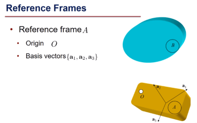
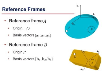
We’re gonna be talking about rigid bodies. The first thing you wanna know about rigid bodies is besides the fact that they’re rigid, you wanna think about modelling them. And in order to model them, we attach reference frames to them. So here I show reference frame A, which is essentially an origin O and a set of axes, x, y, and z. We would also need a set of unit vectors that are parallel to these axes, a1, a2, and a3. So these vectors are mutually orthogonal.

And in fact, it’s these vectors that are more important than the axes. In fact, I’m gonna get rid of those axes and just keep the unit vectors, a1, a2, and a3. You have to remember that these vectors are attached to the rigid body as is the origin O.

Likewise for frame B, we have another set of unit vectors, b1, b2,and b3. And an origin P that’s attached to the rigid body.

So, we have two sets of basis vectors. Each set of basis vectors consists of mutually orthogonal unit vectors. The as are attached to the frame A, the bs are attached to the frame B.

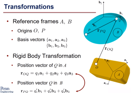
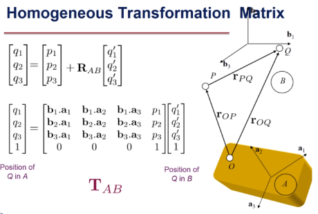
Now I have a different set of components, q1 prime, q2 prime and q3 prime. Clearly, they are different from q1, q2, and q3 because b1, b2, and b3 are different from a1, a2, and a3. And yet, we wanna find a relationship between q1, q2, and q3 on one side and q1 prime, q2 prime, and q3 prime on the other side. This relationship is called a rigid body transformation because you’re talking about the same point. And looking at it from the vantage point of two different frames, each frame attached to a different rigid body.

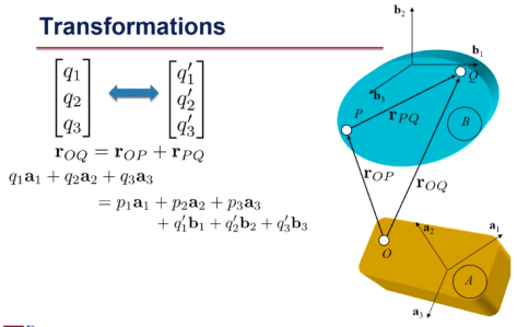
So how do we relate q1, q2, and q3 to q1 prime, q2 prime, and q3 prime? Well, you can write down the vectors pictorially, and you see that immediately that picture suggests that you can use the triangle law of vector addition. The vector from O to Q is simply the sum of the vector from O to P, and the vector from P to Q. I can write this down in terms of components, as we’ve discussed before.

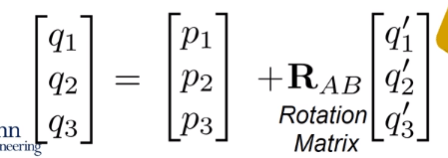
So now, I have a vector equation.I could even try to write this equation in terms of 3 by 1 vectors.

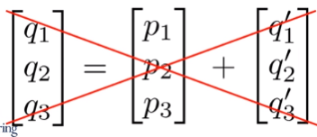
But you cannot simply add these 3 by 1 vectors.

Instead, you should take the vector of components q1 prime, q2 prime, and q3 prime, pre-multiplied by suitable transformation matrix, so that the resulting set of components is along a1, a2, and a3. Well, this transformation is essentially due to a rotation. And the matrix in front is a 3 by 3 rotation matrix. It’s denoted by the boldface symbol R with subscripts A and B. Suggesting that you are transforming components from frame B into frame A.

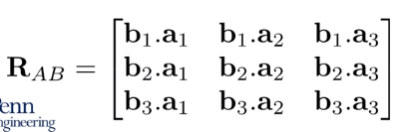
How do you write the components of a rotation matrix? Well, it’s a 3 by 3 matrix, and if you look carefully at the vector equation and the equation with 3 by 1 vectors, you can see that the rotation matrix is simply a collection of dot products or scalar products. You’re taking all possible combinations of the basis vectors, b1, b2, and b3, with the basis vectors a1, a2, and a3. In fact, if you look at the first row, it is simply the components of the basis vector b1 written in frame A.

Now we’re gonna collapse everything into a single matrix, the homogenous transformation matrix. Again, the same equation that essentially describes the triangle law of vector addition in terms of components, components written in terms of a1, a2, and a3. Let’s use homogeneous coordinates where we append the regular xyz coordinates by the number 1 as the fourth element. So this set of four numbers essentially give you a vector which is a representation of the position vector, but in projector coordinates. To relate these two sets of 4 by 1 vectors, all you need is a homogenous transformation matrix that includes elements of the rotation matrix that we’ve just described and the translation from O to P given by the components p1, p2, and p3. The last row, which consists of 0s and 1s, is simply inserted to make sure that the matrix multiplication reflects the triangle law of vector addition.

Well, this 4 by 4 matrix, we’re gonna denote by the boldface symbol T with subscripts A and B. And again, the subscripts denote the fact that you’re transforming position vectors from the second letter, B, to the first letter, A. This is our 4 by 4 homogeneous transformation matrix.

For an example see: Transformation example in Matlab

Written by: Larry Francis Obando – Technical Specialist

Escuela de Ingeniería Eléctrica de la Universidad Central de Venezuela, Caracas.

Escuela de Ingeniería Electrónica de la Universidad Simón Bolívar, Valle de Sartenejas.

Escuela de Turismo de la Universidad Simón Bolívar, Núcleo Litoral.

Contact: Ecuador (Quito, Guayaquil, Cuenca)

WhatsApp: 00593984950376

email: dademuchconnection@gmail.com
Copywriting, Content Marketing, Tesis, Monografías, Paper Académicos, White Papers (Español – Inglés)

Control System Analysis

Control systems are dynamic systems.

Dynamic system definition.

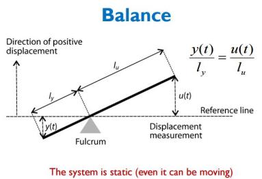
The first thing you must understand in the analysis of control systems is that control systems are dynamic systems. According to Ogata (1987), a system is dynamic when its output in present time depends on its input in the past. If the system output in the present time depends just on an input in the present time, the system is called static. In a dynamic system, the output changes with the time if the system is not in its equilibrium state, while, in a static system, the output keeps constant if the input doesn’t change; i.e. the output changes only when the input changes. See an excellent introduction by Prof. Pedro Albertos from UPV: Systems and Signals Examples.

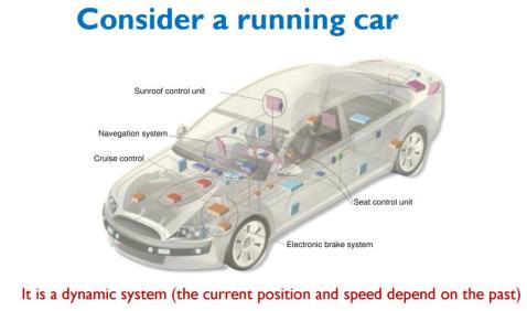
Figures 1 and 2 are examples of static systems and dynamic systems respectively. The first shows the balance relation of a lever supported over a fulcrum. The present value of y(t) depends on the present value of the input u(t). The second shows that the speed and the position of a vehicle depend on an input in the past.


Ejemplo de sistema estático
Figure 1. An example of a static system (Albertos, 2016).

Ejemplo de sistema dinámico

Figura 2. An example of a dynamic system (Albertos, 2016).

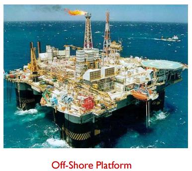
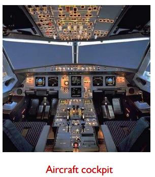
The artificial systems such as the Off-Shore Platform of Figure 3 and the Aircraft cockpit of Figure 4, are also examples of high-complex dynamic systems made by the human beings:


Ejemplo de sistema dinámico. Sistema artificial 1
Figure 3. Artificial system. (Albertos, 2016)


Ejemplo de sistema dinámico. Sistema artificial 2
Figure 4. Artificial system (Albertos, 2016)


The transient response.

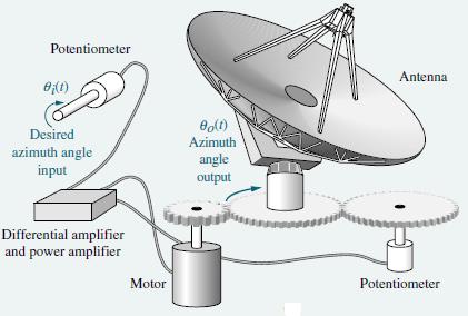
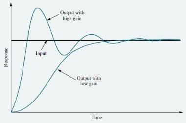
Regarding the control systems, the author Nise defines dynamic systems as follows:  “A control system is dynamic: It responds to an input by undergoing a transient response before reaching a steady-state response that generally resembles the input” (Nise, 2011, p. 10). Figure 5 shows a system to control the position of an antenna. Here, the output is the angular position  (Azimuth Angle), while the input is the signal  sent by the potentiometer. Figure 6 shows the output (blue line) of the system showed in Figure 5, in terms of the transient response and the steady-state response, both for high gain and low gain.


Ejemplo de sistema dinámico. Sistema de control de posición.
Figure 5. Position control system for an Antenna (Nise, 2011)


Ejemplo de sistema dinámico. Respuesta de Sistema de control de posición ejemplo 5.
Figure 6. Transient response and steady-state response for the system of Figure 5.


The goal of the control system of Figure 5 is to place the antenna into the position determined by the input. That´s why the output follows the input. Analyzing Figure 6 we can observe the main characteristic of dynamic systems, which is that, the response in any time after t=0 depends on the input in the past, i.e. the input in t=o determines the output in any time in the future. The transient response is the response of the system before reaching completely the steady-state response (the final value). Looking to the Figure 6, we can find two transient responses. The first one corresponds to a high gain. It generates a lot of fluctuations before the system reaches its steady-state, but it has the advantage of being faster in getting the final value. Here we can image the antenna getting its final position with a fast moving but zigzagging around it. The second one corresponds to a low gain, where there are no fluctuations and we get a very cushioned movement, but the system takes much more time in getting the final value. The selection of one or the other kind of transient response depends on the requirements of the operation and the limits of the system in order to maintain stability.

LTI Systems.

Studying control system implies to obtain as a first step its model. Indeed, before analyzing a control system, we have to develop a mathematical model of a dynamic system.

A mathematical model is perceived as a set of equations representing the dynamic of the system in an exact or approximate way. Such a dynamic, being the system an electrical, a mechanical or a biological one, can be represented by mean of differential equations (Ogata, 2002). In general, resolving a problem requires getting a simple and simplified model in the first stage, in order to visualize the solution by mean of the most practical way. To obtain a simplified model, the control engineer must decide which variable are important and which factors can be ignored.

Once we have an approximate idea of the kind and scope of the solution, the natural or forced response of the system, the model can be optimized and be transformed in one of more complexity, which requires the application of specialized software to be simulated and analyzed, with the aim of obtaining hidden and valuable information.

Talking about making a model, the MIT professor John Sterman shares its philosophy about the efficacy of a model as follows:

“Every model is a representation of a system…But for a model to be useful, it must address a specific problem and must simplify rather than attempt to mirror an entire system in detail…the usefulness of models lies in the fact that they simplify reality, creating a representation of it, we can comprehend…Von Clausewitz famously cautioned that the map is not the territory. It´s a good thing it isn´t: A map as detailed as the territory would be of no use” (Sterman, 2000, p. 89) .

To obtain the equations which set up the models of dynamic systems, the engineers use the laws of the physics applied to the properties of the systems, always searching for the easier path when they are building the model. Among the most useful properties to accomplish this objective, we have the properties of linearity and invariance in time, basically for two main reasons. In the first place, a huge quantity of physical processes, overall those which concern to science, have both properties. In the second place, the linear and time-invariant systems (LTI Systems) are widely accessible in terms of available tools for their analysis. The science of signals and systems has reached a powerful development on these software tools for the systems analysis, allowing people from different academic fields to easily approach to the study of LTI systems (Oppenheim, 1996). That’s why the comprehension of LTI systems becomes the next task at the engineers’ training for the analysis of control systems.

  Analysis and Design definition.

Before getting deeper on the characteristics of the LTI Systems, the engineers need to strictly define the basic areas of their work as control engineers [1]: the analysis, the design and the synthesis of systems.

Analysis: it is the study of the functioning of a system at specific conditions, which mathematical model is known. Generally, they are varied, the values of the parameters involved in the mathematical models in order to observe the different responses and from there to get conclusions. As the analysis depends on the mathematical model, it is independent of the kind of the system studied, being this mechanical, electrical or hydraulic.

Design: given a specific task, it is the process whereby we can find the system which accomplishes that task.  Usually, it is not a direct process and requires essay and error. The design implies to make it clear the requirements of the system, typically given in qualitative and quantitative terms. Subsequently, the engineer uses the synthesis. Once he has a model, the engineer analyzes the system so foresee the compliance of the requirements by mean of computerized simulation. By applying essay and error, the engineer modifies the model until it approximately meets the desired result. If it is possible, the engineer builds a prototype and continues the analysis until it meets the final goal.

Synthesis: it is the use of a specific procedure to find a system which works in a specific way. In this case, the characteristics of the system are postulated at the beginning and afterward the engineer uses several mathematical techniques to come up with the right system.

There are therefore two methods for designing (Distefano et al, 1995):

  1. Design from the analysis: it is made by mean of the modification of the characteristics of a system which already exists;
  2. Design from the synthesis: it is the definition of a system starting from its specifications.

In relation to control systems, Nise defines the functions of an engineer as follows:“…we discuss three major objectives of systems analysis and design: producing the desired transient response, reducing steady-state error, and achieving stability” (Nise, 2011, p. 10).