We discuss two ways to improve the steady-state error of a feedback control system using cascade compensation. One objective of this design is to improve the steady-state error without appreciably affecting the transient response.
Improving Transient Response - Compensation
We have seen before that setting the gain at a particular value on the root locus yields the transient response dictated by the poles at that point on the root locus. Thus, we are limited to those responses that exist along the root locus. (See Sketching Root Locus with Matlab – Control Systems)
Unfortunately, most of the time the overshoot specification for designing control systems exceed the posibilities of the current root locus. What can we do then?
Rather than change the existing system, we augment, or compensate, the system with additional poles and zeros, so that the compensated system has a root locus that goes through the desired pole location for some value of gain. One of the advantages of compensating a system in this way is that additional poles and zeros can be added at the low-power end of the system before the plant. We should evaluate the transient response through simulation after the design is complete to be sure the requirements have been met.
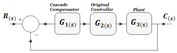
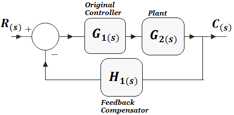
There are two configurations of compensation mostly used in control systems design: cascade compensation and feedback compensation. These methods are modeled in Figure 1 and Figure 2:
Figure 1. Cascade Compensation of a control system.
With cascade compensation, the compensating network, G1(s), is placed at the low-power end of the forward path in cascade with the plant, Figure 1.
Figure 2. Feedback Compensation of a control system.
With feedback compensation, the compensator, H1(s), is placed in the feedback path, Figure 2.
Both methods change the open-loop poles and zeros, thereby creating a new root locus that goes through the desired closed-loop pole location.
Cascade Compensation - PI Controller
Steady-state error can be improved by placing an open-loop pole at the origin,
because this increases the system type by one. For example, a Type 0 system
responding to a step input with a finite error, will responds with zero error if the system
type is increased by one. But, we want to do this without affecting the transient response.
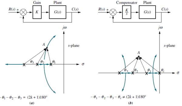
However, if we add a pole at the origin to increase the system type, the angular contribution of the open-loop poles at hypothetical point A is no longer 180, and the root locus no longer goes through point A, as shown in Figure 3.a and 3.b:
Figure 3.
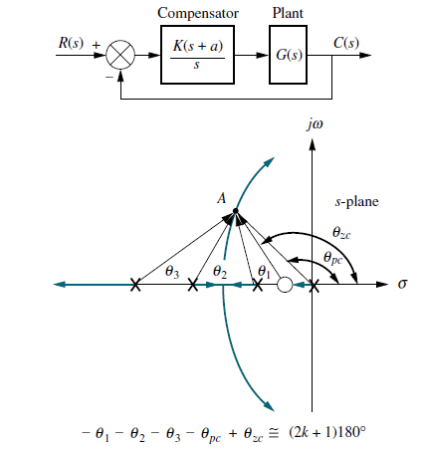
To solve the problem, we also add a zero close to the pole at the origin, as shown
in Figure 4:
Figure 4.
Now the angular contribution of the compensator zero and compensator pole cancel out, point A is still on the root locus, and the system type has been increased. That is how we can improve the steady-state error without affecting the transient response.
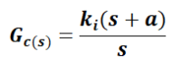
A compensator with a pole at the origin and a zero close to the pole is called an ideal integral compensator, or Proportional-plus-Integral PI compensator, which transfer function Gc(s) is:
Next example allows to find how PI compensation works.
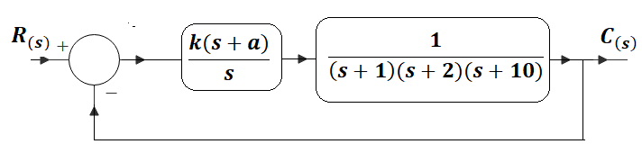
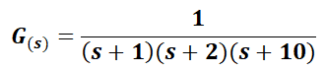
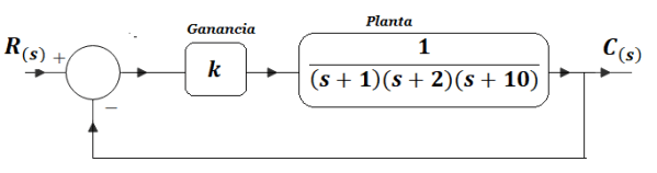
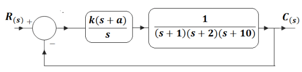
For control system of Figure 5, it is required to reduce steady-state error to zero, through a PI controller, keeping damping at ξ=0.173. The plant transfer function is G(s) and its original controller is represented by the gain k:
Figure 5.
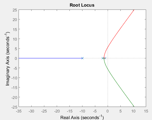
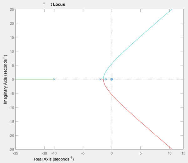
The first step is to evaluate the system before the compensation, then to find the location of the two closed-loop second-order dominant poles in order to get the damping requiered by the design specifications.
Figure 6 shows the Root-Locus of the system before compensation:
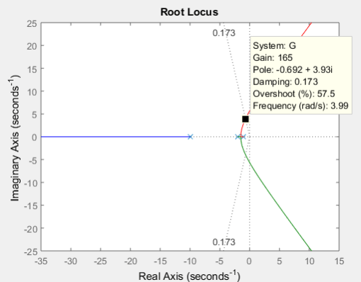
Using the damping line in Matlab, we can find the intersection point between the root-locus and the value ξ=0.173, as we can see in Figure 7:
>> z=0.173;
>> sgrid(z,0)
Figure 7.
The intersection of Figure 7 shows us that adjusting the gain to k=165 of the original controller, we obtain the damping requiered: ξ=0.173. We also see in Figure 7 that the closed-loop second-order dominant poles s1 and s2, before compensation are:
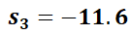
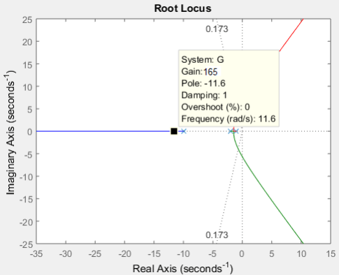
Now we look for the third pole in the root locus. In Figure 8 we must set the same gain k=165 at the third pole line, in consequence s3 is located at:
Figure 8.
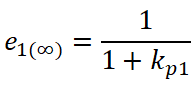
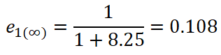
With k=165 we calculate the steady-state error e1(∞) for a step input, before compensation:
Where kp1 the position constant before compensation:
Where kG(s) is the system forward transfer function multiplied by the adjusted gain, before compensation, as in Figure 5. Therefore:
We add a PI controller in cascade into the system, as in Figure 9:
Figure 9.
Here, we have matched the gain constant of the compensator with the original gain constant, that is to say k=ki. The constant a is determined by the location of compensator zero, wich must be near the compensator pole. That is why we set the compensator zero at s=-0.1 , that is to say a=0.1. The root locus of this compensated system is in Figure 10:
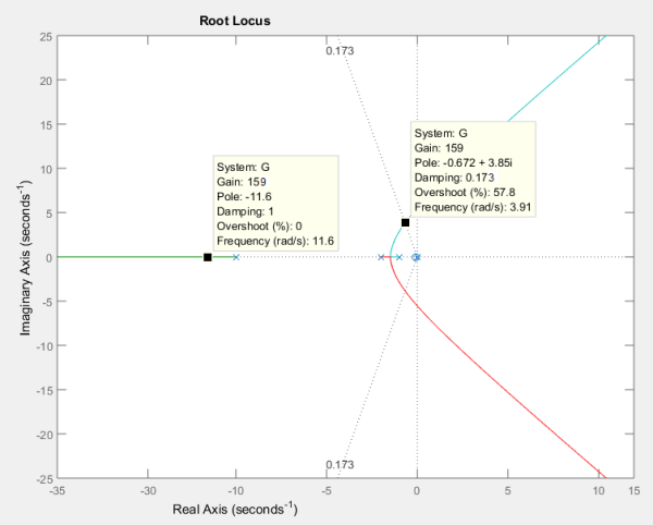
In view of the fact that we want to maintain the transient response as unchanged as possible, in Figure 11 we draw the damping line in the root locus and search for the point of intersection between the lines of the root locus and ξ=0.173:
>> z=0.173;
>> sgrid(z,0);
Figure 11.
Adjusting the gain to k=159 in Figure 11, we obtain the damping ξ=0.173. We see that closed-loop second-order dominant poles s1 and s2, after compensation, are:
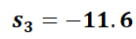
Looking for the third pole in the root locus, we must set the gain k=159 at the third pole line. After that, s3 is located at:
These results show that approximately the values of the 3 poles before and after the PI compensation have been conserved, indicating a similar transient response after correcting the error in steady state from 0.108 to 0, as shwon later.
The forward transfer function G2(s) of the system after compensation is:
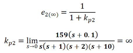
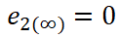
One more time, we calculate steady-state error e2(∞) for a step input, after compensation:
In consequence:
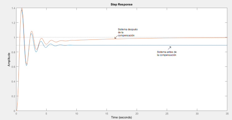
Figure 12 compares the step response of the closed-loop system before and after compensatio PI:
Figure 12 shows that through PI compensation we have managed to improve the steady-state error without considerably modifying the transient response of the original system.
Compensación en Cascada - Lag Compensation
In construction…
Source :
Control Systems Engineering, Nise
Written by Prof. Larry Francis Obando – Technical Specialist – Educational Content Writer
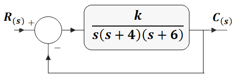
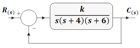
Given the system of Figure 1, design a PD compensator to yield a 16% overshoot, with a threefold reduction in settling time (one-third of the uncompensated system’s settling time).
Figure 1
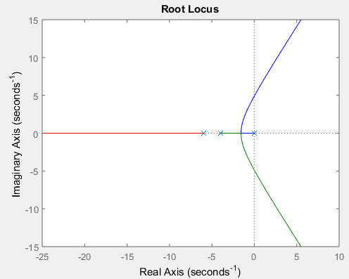
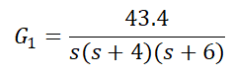
Let us first evaluate the performance of the uncompensated system. The root locus for the uncompensated system is shown in Figure 2:
>> s=tf(‘s’);
>> G=1/(s*(s+4)*(s+6));
Figure 2
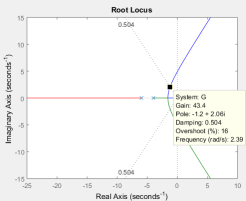
Since 16% overshoot is equivalent to ξ=0.504, we search along that damping ratio line in Figure 3:
>> z=0.504;
>> sgrid(z,0);
Figure 3
According to Figure 3, adjusting the gain to k=43.4 we get ξ=0.504 and a natural frequency ω=2.39 rad/s.
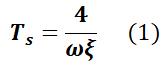
Based upon a second-order approximation, we can use the 2% criteria and calculate the settling-time Ts1before the compensation, as a function of the naural frequency ω and the damping ξ, by means of the following equation:
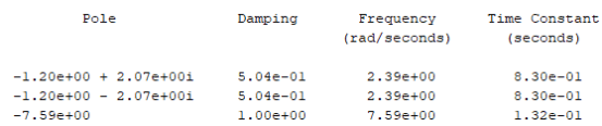
Simulation of Figure 3 generates the necessary values for equation (1), so that:
In the other hand, the value of the factor ω*ξ=1.2045 matches the real part σ of closed-loop second-order dominant poles, as we can see in Figure 3 or by the following command in Matlab, taking into consideration that the straight-forward transfer function is now G1:
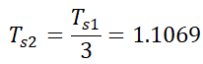
The desig requirements ask for an 16% overshoot and a reduction of the settling-time of 1/3 after compensation. So, the settling-time Ts2after compensation is:
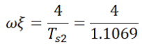
Using equation (1) we can know the value of the factor ω*ξ after compensation:
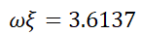
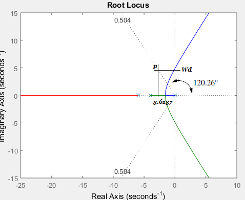
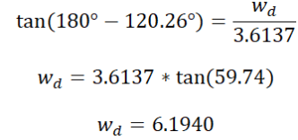
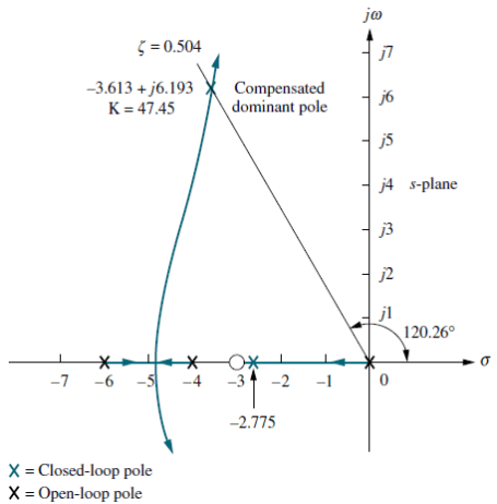
That is to say, the real part of second-order dominant poles after compensation is σ=3.6137. To find the imaginary part wd we use the root-locus of Figure 4:
Figure 4.
Consequently, after compensation the second-order dominant poles must be located at p=-3.6137+j6.1940.
Now, to evaluate the whole system we will use point p as a test point.
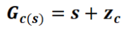
PD compensation consists of a cascaded controller with a Gc(s) transfer funcion that is:
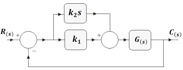
The configuration of such a controller is:
Figure 5.
Next step is to design the location of Zero zc using the test point p and finding the equivalent values for k1and k2.
The result is the sum of the angles to the design point of all the poles and zeros of the compensated system except for those of the compensator zero itself. The difference between the result obtained and 180 is the angular contribution required of the compensator zc es:
The geometry is shown in Figura 6, where we can get the real part of zc by means of the following formula:
Figure 6.
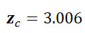
From where:
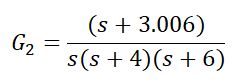
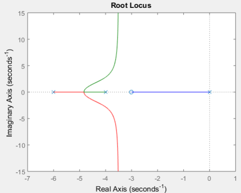
Now, we study the root-locus of Figure 7, where the forward-path transfer function is G2:
>> G2=(s+3.006)/(s*(s+4)*(s+6));
>> rlocus(G2)
Figure 7.
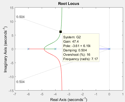
According to Figure 8, adjusting the gain k=47.4 we keep ξ=0.504, an overshoot16%, the second-order dominant pole s=-3.6137+j6.1940, at a natural frequency ω=7.17 rad/s.
>> z=0.504;
>> sgrid(z,0);
Figure 8.
With this new data, we evaluate the settling-time Ts2 after compensation:
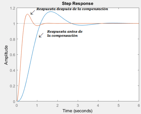
It shows that we have achieved the design goal. Figure 9 compares the response of the closed-loop system to an step input before and after PD compensation:
The response of Figure 9 shows a considerable improvement in the settling-time and, in general, the compensation allows a faster system with an overshoot that does not vary much. Before compensation, Ts=3.4712 s. After compensation, Ts=1.1527 s.
An alternative design process in Matlab
Use MATLAB, the Control System Toobox, and the following steps to use SISOTOOL to perform the design of last Example.
Type sisotool in the MATLAB Command Window.
Select Import in the File menu of the SISO Design for SISO Design Task Window.
In the Data field for G, type zpk([],[0,-4,-6],1) and hit ENTER on the keyboard. Click OK.
On the Edit menu choose SISO Tool Preferences . . . and select Zero/pole/gain: under the Options tab. Click OK.
Right-click on the root locus white space and choose Design Requirements/New . . .
Choose Percent overshoot and type in 16. Click OK.
Right-click on the root locus white space and choose Design Requirements/New . . .
Choose Settling time and click OK.
Drag the settling time vertical line to the intersection of the root locus and 16%
overshoot radial line.
Read the settling time at the bottom of the window.
Drag the settling time vertical line to a settling time that is 1/3 of the value
found in Step 9.
Click on a red zero icon in the menu bar. Place the zero on the root locus real axis by clicking again on the real axis.
Left-click on the real-axis zero and drag it along the real axis until the root locus intersects the settling time and percent overshoot lines.
Drag a red square along the root locus until it is at the intersection of the root locus,
settling time line, and the percent overshoot line.
Click the Compensator Editor tab of the Control and Estimation Tools Manager window to see the resulting compensator, including the gain.
Source:
Control Systems Engineering, Nise
Written by: Larry Francis Obando – Technical Specialist – Educational Content Writer.
Mentoring Académico / Empresarial / Emprendedores
Copywriting, Content Marketing, Tesis, Monografías, Paper Académicos, White Papers (Español – Inglés)
Escuela de Ingeniería Eléctrica de la Universidad Central de Venezuela, Caracas.
Escuela de Ingeniería Electrónica de la Universidad Simón Bolívar, Valle de Sartenejas.
Escuela de Turismo de la Universidad Simón Bolívar, Núcleo Litoral.
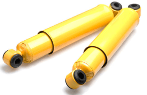
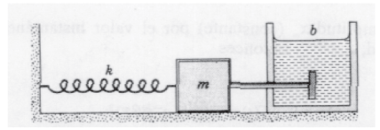
The basic elements of any mechanical system are the mass, the spring and the shock absorber, or damper. The study of movement in mechanical systems corresponds to the analysis of dynamic systems. In Robotics, for example, the word Forward Dynamic refers to what happens to actuators when we apply certain forces and torques to them.
The mass, the spring and the damper are basic actuators of the mechanical systems.
Consequently, to control the robot it is necessary to know very well the nature of the movement of a mass-spring-damper system.
In addition, this elementary system is presented in many fields of application, hence the importance of its analysis. Again, in robotics, when we talk about Inverse Dynamic, we talk about how to make the robot move in a desired way, what forces and torques we must apply on the actuators so that our robot moves in a particular way.
I recommend the book «Mass-spring-damper system, 73 Exercises Resolved and Explained» I have written it after grouping, ordering and solving the most frequent exercises in the books that are used in the university classes of Systems Engineering Control, Mechanics, Electronics, Mechatronics and Electromechanics, among others.
If you need to acquire the problem solving skills, this is an excellent option to train and be effective when presenting exams, or have a solid base to start a career on this field. Take a look at the Index at the end of this article.
Before performing the Dynamic Analysis of our mass-spring-damper system, we must obtain its mathematical model. This is the first step to be executed by anyone who wants to know in depth the dynamics of a system, especially the behavior of its mechanical components.
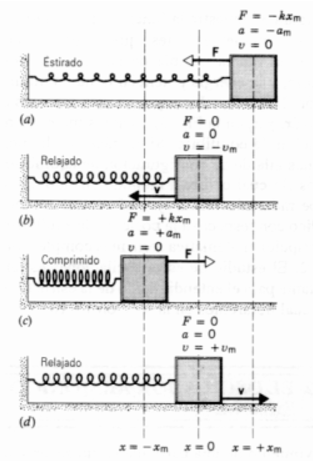
We will begin our study with the model of a mass-spring system.
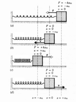
This is convenient for the following reason. All the mechanical systems have a nature in their movement that drives them to oscillate, as when an object hangs from a thread on the ceiling and with the hand we push it. Or a shoe on a platform with springs. It is good to know which mathematical function best describes that movement.
But it turns out that the oscillations of our examples are not endless. There is a friction force that dampens movement. In the case of the object that hangs from a thread is the air, a fluid. So after studying the case of an ideal mass-spring system, without damping, we will consider this friction force and add to the function already found a new factor that describes the decay of the movement.
Mass-Spring System.
Figure 5
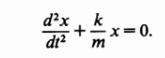
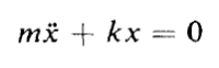
The dynamics of a system is represented in the first place by a mathematical model composed of differential equations. In the case of the mass-spring system, said equation is as follows:
This equation is known as the Equation of Motion of a Simple Harmonic Oscillator. Let’s see where it is derived from.
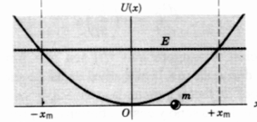
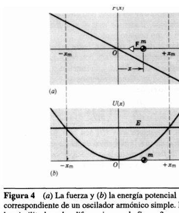
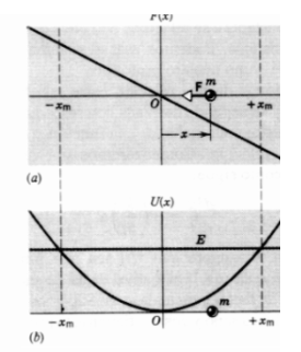
If our intention is to obtain a formula that describes the force exerted by a spring against the displacement that stretches or shrinks it, the best way is to visualize the potential energy that is injected into the spring when we try to stretch or shrink it. The following graph describes how this energy behaves as a function of horizontal displacement:
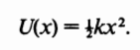
As the mass mof the previous figure, attached to the end of the spring as shown in Figure 5, moves away from the spring relaxation point x = 0 in the positive or negative direction, the potential energy U (x) accumulates and increases in parabolic form, reaching a higher value of energy where U (x) = E, value that corresponds to the maximum elongation or compression of the spring. The mathematical equation that in practice best describes this form of curve, incorporating a constant k for the physical property of the material that increases or decreases the inclination of said curve, is as follows:
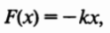
The force is related to the potential energy as follows:
Therefore:
It makes sense to see that F (x) is inversely proportional to the displacement of mass m. Because it is clear that if we stretch the spring, or shrink it, this force opposes this action, trying to return the spring to its relaxed or natural position. For that reason it is called restitution force. The above equation is known in the academy as Hooke’s Law, or law of force for springs. The following is a representative graph of said force, in relation to the energy as it has been mentioned, without the intervention of friction forces (damping), for which reason it is known as the Simple Harmonic Oscillator. It is important to emphasize the proportional relationship between displacement and force, but with a negative slope, and that, in practice, it is more complex, not linear.
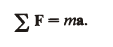
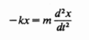
This equation tells us that the vectorial sum of all the forces that act on the body of mass m, is equal to the product of the value of said mass due to its acceleration acquired due to said forces. Considering that in our spring-mass system, ΣF = -kx, and remembering that acceleration is the second derivative of displacement, applying Newton’s Second Law we obtain the following equation:
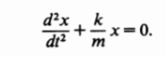
Fixing things a bit, we get the equation we wanted to get from the beginning:
This equation represents the Dynamics of an ideal Mass-Spring System.
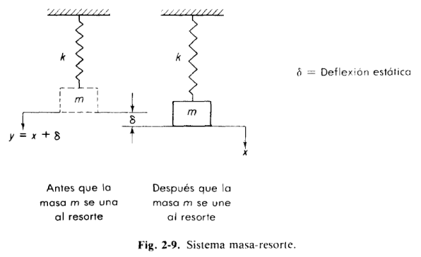
Apart from Figure 5, another common way to represent this system is through the following configuration:
:
In this case we must consider the influence of weight on the sum of forces that act on the body of mass m. The weight P is determined by the equation P = m.g, where g is the value of the acceleration of the body in free fall.
If the mass is pulled down and then released, the restoring force of the spring acts, causing an acceleration ÿ in the body of mass m. We obtain the following relationship by applying Newton:
If we implicitly consider the static deflection, that is, if we perform the measurements from the equilibrium level of the mass hanging from the spring without moving, then we can ignore and discard the influence of the weight P in the equation. If we do y = x, we get this equation again:
Mass-spring-damper System
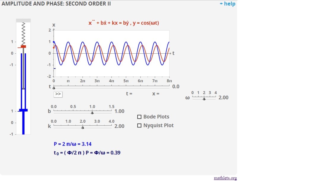
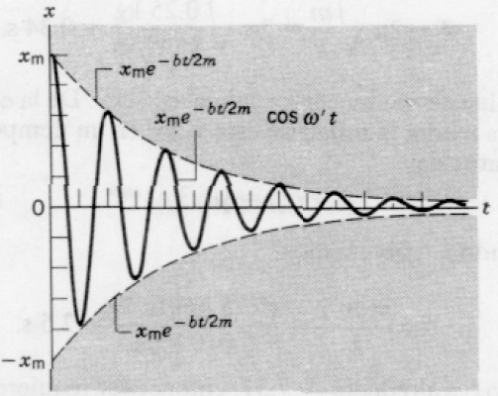
If there is no friction force, the simple harmonic oscillator oscillates infinitely. In reality, the amplitude of the oscillation gradually decreases, a process known as damping, described graphically as follows:
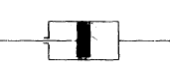
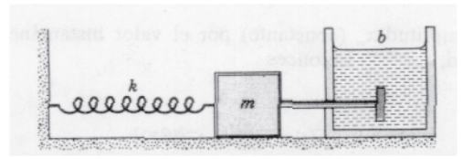
The displacement of an oscillatory movement is plotted against time, and its amplitude is represented by a sinusoidal function damped by a decreasing exponential factor that in the graph manifests itself as an envelope. The friction force Fv acting on the Amortized Harmonic Movement is proportional to the velocity Vin most cases of scientific interest. This force has the form Fv = bV, where b is a positive constant that depends on the characteristics of the fluid that causes friction. This friction, also known as Viscose Friction, is represented by a diagram consisting of a piston and a cylinder filled with oil:
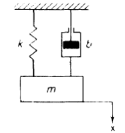
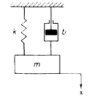
The most popular way to represent a mass-spring-damper system is through a series connection like the following:
Figura 6
As well as the following:
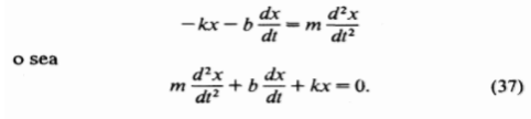
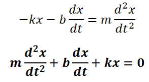
In both cases, the same result is obtained when applying our analysis method. Considering Figure 6, we can observe that it is the same configuration shown in Figure 5, but adding the effect of the shock absorber. Applying Newton’s second Law to this new system, we obtain the following relationship:
This equation represents the Dynamics of a Mass-Spring-Damper System.
Laplace Transform of a Mass-Spring-Damper System
A solution for equation (37) is presented below:
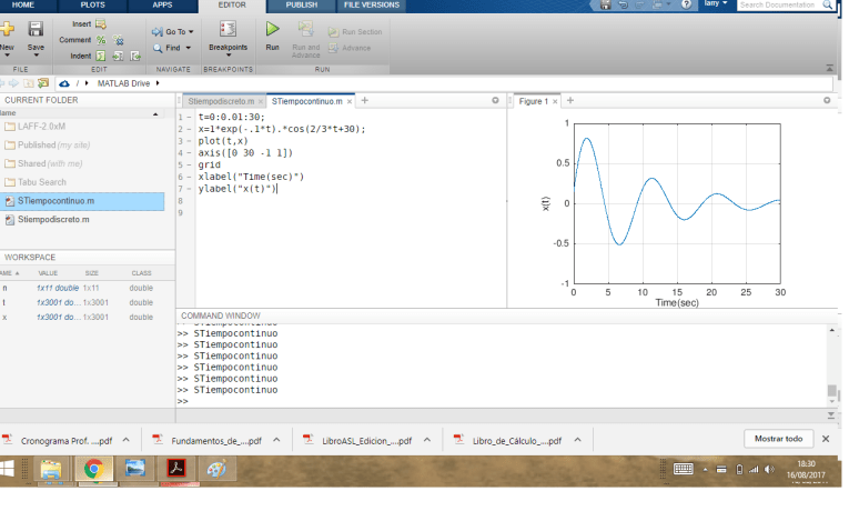
Equation (38) clearly shows what had been observed previously. An example can be simulated in Matlab by the following procedure:
The shape of the displacement curve in a mass-spring-damper system is represented by a sinusoid damped by a decreasing exponential factor. It is important to understand that in the previous case no force is being applied to the system, so the behavior of this system can be classified as «natural behavior» (also called homogeneous response). Later we show the example of applying a force to the system (a unitary step), which generates a «forced behavior» that influences the final behavior of the system that will be the result of adding both behaviors (natural + forced). Remark: When a force is applied to the system, the right side of equation (37) is no longer equal to zero, and the equation is no longer homogeneous.
The solution for the equation (37) presented above, can be derived by the traditional method to solve differential equations. However, this method is impractical when we encounter more complicated systems such as the following, in which a force f(t) is also applied:
Figura 7
The need arises for a more practical method to find the dynamics of the systems and facilitate the subsequent analysis of their behavior by computer simulation. The Laplace Transform allows to reach this objective in a fast and rigorous way.
In equation (37) it is not easy to clear x(t), which in this case is the function of output and interest. A differential equation can not be represented either in the form of a Block Diagram, which is the language most used by engineers to model systems, transforming something complex into a visual object easier to understand and analyze.The first step is to clearly separate the output function x(t), the input function f(t) and the system function (also known as Transfer Function), reaching a representation like the following:
r(t)=f(t), c(t)=x(t)
The Laplace Transform consists of changing the functions of interest from the time domain to the frequency domain by means of the following equation:
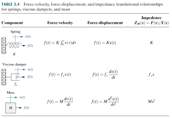
The main advantage of this change is that it transforms derivatives into addition and subtraction, then, through associations, we can clear the function of interest by applying the simple rules of algebra. In addition, it is not necessary to apply equation (2.1) to all the functions f(t) that we find, when tables are available that already indicate the transformation of functions that occur with great frequency in all phenomena, such as the sinusoids (mass system output, spring and shock absorber) or the step function (input representing a sudden change). In the case of our basic elements for a mechanical system, ie: mass, spring and damper, we have the following table:
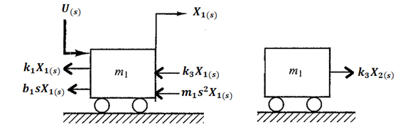
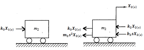
That is, we apply a force diagram for each mass unit of the system, we substitute the expression of each force in time for its frequency equivalent (which in the table is called Impedance, making an analogy between mechanical systems and electrical systems) and apply the superposition property (each movement is studied separately and then the result is added).
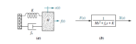
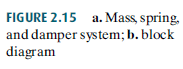
Figure 2.15 shows the Laplace Transform for a mass-spring-damper system whose dynamics are described by a single differential equation:
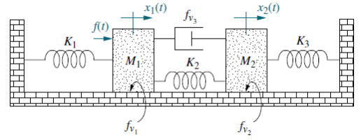
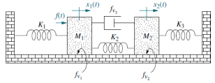
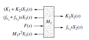
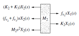
The system of Figure 7 allows describing a fairly practical general method for finding the Laplace Transform of systems with several differential equations. First the force diagram is applied to each unit of mass:
For Figure 7 we are interested in knowing the Transfer Function G(s)=X2(s)/F(s).
Arranging in matrix form the equations of motion we obtain the following:
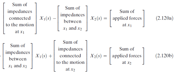
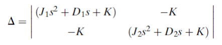
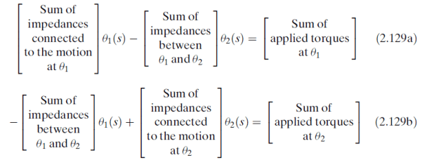
Equations (2.118a) and (2.118b) show a pattern that is always true and can be applied to any mass-spring-damper system:
The immediate consequence of the previous method is that it greatly facilitates obtaining the equations of motion for a mass-spring-damper system, unlike what happens with differential equations. In addition, we can quickly reach the required solution. In the case of our example:
Where:
These are results obtained by applying the rules of Linear Algebra, which gives great computational power to the Laplace Transform method.
Application examples ...under construction
Example 1.
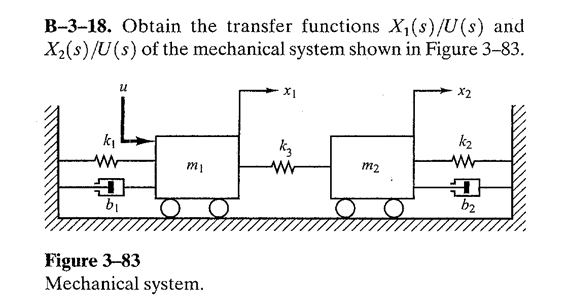
Exercise B318, Modern_Control_Engineering, Ogata 4t p 149 (162),
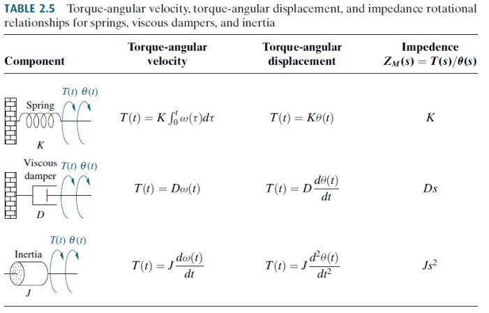
So far, only the translational case has been considered. In the case that the displacement is rotational, the following table summarizes the application of the Laplace transform in that case:
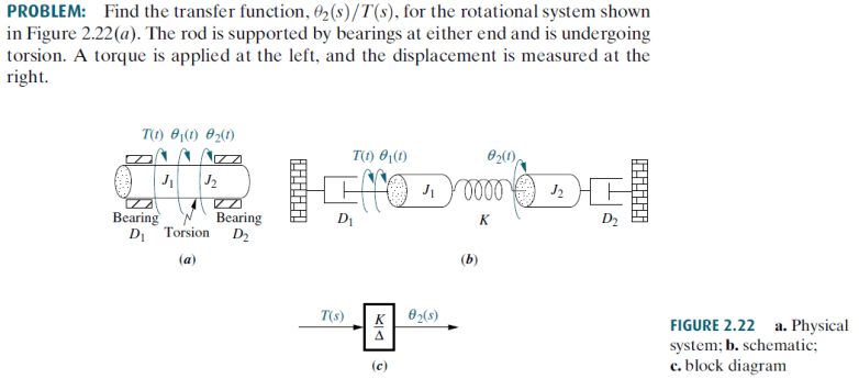
Example:
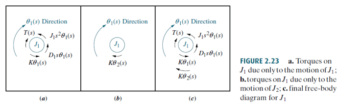
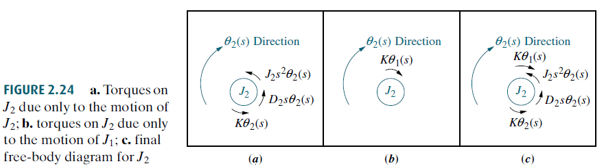
The following figures illustrate how to perform the force diagram for this case:
Therefore:
Being:
We observe that again it is true that:
Bibliography
:
Robert Resnick, tomo1
Dinamica_de_Sistemas, Katsuhiko Ogata
Control Systems Engineering, Norman Nise
Sistemas de Control Automatico, Benjamin Kuo
Ingenieria de Control Moderna, 3° ED. – Katsuhiko Ogata
Attention!
I recommend the book «Mass-spring-damper system, 73 Exercises Resolved and Explained» I have written it after grouping, ordering and solving the most frequent exercises in the books that are used in the university classes of Systems Engineering Control, Mechanics, Electronics, Mechatronics and Electromechanics, among others.
If you need to acquire the problem solving skills, this is an excellent option to train and be effective when presenting exams, or have a solid base to start a career on this field.
INDEX
Preface ii
Introduction iii
Chapter 1———————————————————- 1
o Mass-spring-damper System (translational mechanical system)
Chapter 2———————————————————- 51
o Mass-spring-damper System (rotational mechanical system)
Chapter 3———————————————————- 76
o Mechanical Systems with gears
Chapter 4———————————————————- 89
o Electrical and Electronic Systems
Chapter 5——————————————————— 114
o Electromechanical Systems – DC Motor
Chapter 6——————————————————— 144
o Liquid level Systems
Chapter 7——————————————————— 154
o Linearization of nonlinear Systems
References——————————————————- 164
Attention!
If what you need is to determine the Transfer Function of a System … We deliver the answer in two hours or less, depending on the complexity. In digital Contact us, immediate response, solve and deliver the transfer function of mass-spring-damper systems, electrical, electromechanical, electromotive, liquid level, thermal, hybrid, rotational, non-linear, etc. Optional, Representation in State Variables. Simulation in Matlab, Optional, Interview by Skype to explain the solution.
WhatsApp +34633129287, Inmediate attention !!
email: dademuchconnection@gmail.com
Written by Prof. Larry Francis Obando – Technical Specialist – Educational Content Writer
Mentoring Académico / Emprendedores / Empresarial
Copywriting, Content Marketing, Tesis, Monografías, Paper Académicos, White Papers (Español – Inglés)
Escuela de Ingeniería Electrónica de la Universidad Simón Bolívar, USB Valle de Sartenejas.
Escuela de Ingeniería Eléctrica de la Universidad Central de Venezuela, UCV CCs
Escuela de Turismo de la Universidad Simón Bolívar, Núcleo Litoral.
Die Grundelemente eines jeden mechanischen Systems sind die Masse, die Feder und der Stoßdämpfer. Das Studium der Bewegung in mechanischen Systemen entspricht der Analyse dynamischer Systeme. In der Robotik zum Beispiel bezieht sich das Wort Vorwärtsdynamik darauf, was mit Aktuatoren passiert, wenn wir bestimmte Kräfte und Drehmomente auf sie anwenden.
Die Masse, die Feder, der Stoßdämpfer sind elementare Aktuatoren eines mechanischen Systems.
Um den Roboter zu steuern, ist es folglich notwendig, die Art der Bewegung eines Masse-Feder-Dämpfer-Systems sehr gut zu kennen.
Darüber hinaus wird dieses elementare System in vielen Anwendungsbereichen vorgestellt, daher die Wichtigkeit seiner Analyse. Wenn wir in der Robotik über Inverse Dynamic sprechen, sprechen wir darüber, wie man den Roboter auf eine gewünschte Art und Weise bewegt, welche Kräfte und Drehmomente wir auf die Aktoren anwenden müssen, damit sich unser Roboter auf eine bestimmte Art bewegt.
Bevor wir die dynamische Analyse unseres Masse-Feder-Dämpfer-Systems durchführen, müssen wir sein mathematisches Modell erhalten. Dies ist der erste Schritt für jeden, der die Dynamik eines Systems, insbesondere das Verhalten seiner mechanischen Komponenten, genau kennenlernen möchte.
Wir werden unsere Studie mit dem Modell eines Masse-Feder-Systems beginnen.
Dies ist aus folgendem Grund praktisch. Alle mechanischen Systeme haben eine Art in ihrer Bewegung, die sie zum Schwingen bringt, etwa wenn ein Gegenstand an einem Faden an der Decke hängt und mit der Hand, die wir drücken. Oder ein Schuh auf einer Plattform mit Federn. Es ist gut zu wissen, welche mathematische Funktion diese Bewegung am besten beschreibt.
Masse-Feder-System.
Abbildung 5
Die Dynamik eines Systems wird in erster Linie durch ein mathematisches Modell dargestellt, das aus Differentialgleichungen besteht. Im Falle des Masse-Feder-Systems ist diese Gleichung wie folgt:
Diese Gleichung ist als Bewegungsgleichung eines einfachen harmonischen Oszillators bekannt. Mal sehen, woher es stammt.
Wenn wir eine Formel erhalten wollen, die die Kraft beschreibt, die eine Feder gegen die Verschiebung ausübt, die sie dehnt oder schrumpft, ist es am besten, die potentielle Energie zu visualisieren, die in die Feder injiziert wird, wenn wir sie dehnen oder schrumpfen. Die folgende Grafik beschreibt, wie sich diese Energie als Funktion der horizontalen Verschiebung verhält:
Wenn sich die Masse m der vorhergehenden Figur, die an dem Ende der Feder angebracht ist, wie in Abbildung 5 gezeigt, von dem Federrelaxationspunkt x = 0 weg in die positive oder negative Richtung bewegt, sammelt sich die potentielle Energie U (x)an und steigt in parabolischer Form an und erreicht einen höheren Energiewert, wobei U(x) = E, Wert, der der maximalen Dehnung oder Kompression der Feder entspricht. Die mathematische Gleichung, die in der Praxis diese Kurvenform am besten beschreibt und eine Konstante k für die physikalische Eigenschaft des Materials enthält, die die Steigung der Kurve erhöht oder verringert, ist die folgende:
Die Kraft ist auf folgende Weise mit der potentiellen Energie verbunden:
Deshalb:
Es ist sinnvoll zu sehen, dass F (x) umgekehrt proportional zur Verschiebung der Masse m ist. Denn es ist klar, dass, wenn wir die Feder dehnen oder schrumpfen, diese Kraft dieser Aktion entgegenwirkt und versucht, die Feder in ihre entspannte oder natürliche Position zurückzubringen. Aus diesem Grund heißt es Restitutionskraft. Die obige Gleichung ist in der Akademie als Hookes Gesetz oder Kraftgesetz für Federn bekannt. Das Folgende ist ein repräsentatives Diagramm dieser Kraft in Bezug auf die Energie, wie sie erwähnt wurde, ohne den Eingriff von Reibungskräften (Dämpfung), weshalb sie als der einfache harmonische Oszillator bekannt ist. Es ist wichtig, die proportionale Beziehung zwischen Verschiebung und Kraft zu betonen, aber mit einer negativen Steigung, und das ist in der Praxis komplexer, nicht linear.
Diese Gleichung sagt uns, dass die vektorielle Summe aller Kräfte, die auf den Körper der Masse m einwirken, gleich dem Produkt des Wertes der Masse aufgrund ihrer Beschleunigung ist, die aufgrund der Kräfte erhalten wird. Mit Newtons zweitem Gesetz erhalten wir die folgende Gleichung:
Das ist:
Diese Gleichung repräsentiert die Dynamik eines idealen Masse-Feder-Systems.
System Masse-Feder-Stoßdämpfer
Wenn keine Reibungskraft vorhanden ist, oszilliert der einfache harmonische Oszillator unendlich. In Wirklichkeit nimmt die Amplitude der Oszillation allmählich ab, ein Prozess, der als Dämpfung bekannt ist und im folgenden graphisch beschrieben wird:
Die Verschiebung einer oszillierenden Bewegung ist gegen die Zeit aufgetragen, und ihre Amplitude wird durch eine sinusförmige Funktion dargestellt, die durch einen abnehmenden Exponentialfaktor gedämpft wird, der in dem Graphen als eine Hüllkurve erscheint. Die Reibungskraft Fv, die auf die amortisierte harmonische Bewegung einwirkt, ist in den meisten Fällen von wissenschaftlichem Interesse proportional zur Geschwindigkeit V. Diese Kraft hat die Form Fv = bV, wobei b eine positive Konstante ist, die unter anderem von den Eigenschaften des Fluids abhängt, das Reibung verursacht. Diese Reibung, auch bekannt als Viskosereibung, wird durch ein Diagramm dargestellt, das aus einem Kolben und einem mit Öl gefüllten Zylinder besteht:
Die gängigste Art, ein Masse-Feder-Dämpfer-System darzustellen, ist eine Reihenschaltung wie folgt:
Abbildung 6
Sowie die folgenden:
In beiden Fällen wird das gleiche Ergebnis bei Anwendung unserer Analysemethode erhalten. Wenn man Fig. 6 betrachtet, kann man sehen, dass dieselbe Konfiguration wie in Fig. 5 gezeigt ist, jedoch die Wirkung des Stoßdämpfers hinzugefügt wird. Indem wir Newtons zweites Gesetz auf dieses neue System anwenden, erhalten wir die folgende Beziehung:
Diese Gleichung repräsentiert die Dynamik eines Massen-Feder-Schock-Systems.
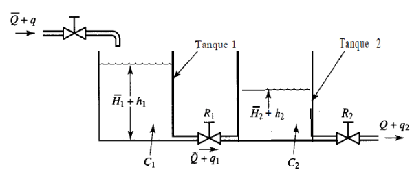
We take into account the liquid-level system of Figure 3-23.
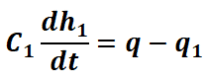
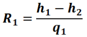
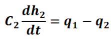
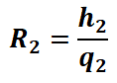
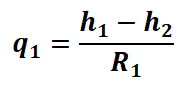
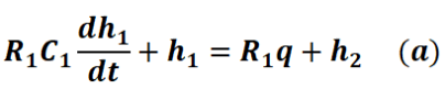
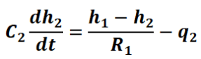
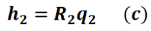
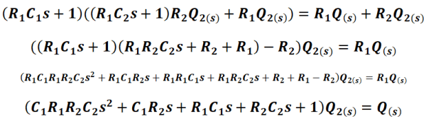
In accordance with the definitions of the previous article (Dinámica de un sistema de nivel de líquidos), we focus on the capacitances C1 and C2, as well as on the resistors R1 and R2. Thus, the dynamics of this system is determined by the following equations:
From here we can obtain the transfer function depending on what variables we define as input and output. For example, suppose the input to the system is q and the output variable is q2,so to find the transfer function of the system we execute the following operations:
So:
That is to say:
In the other hand:
That is:
Also:
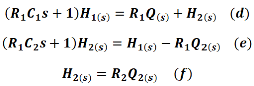
Applying Laplace to equations a, b and c, we obtain:
Clearing H1(s) of eand substituting this value in d we obtain:
An due to f the latter is:
The transfer function of the system is:
Written by: Larry Francis Obando – Technical Specialist – Educational Content Writer.
Suppose we have a system represented by the following function: Our task is to linearize f (x) around xo = π / 2. As: We find the following values and substitute them in the previous equation: Then we can represent our nonlinear system by means of the following negative line equation:
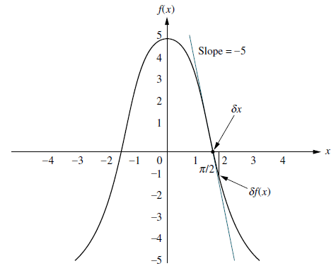
The result of the linearization of f (x) around xo = π / 2 can be seen in Figure 2.48:
Linearize a differential equation
Suppose now that our system is represented by the following differential equation: The presence of the term cosx makes the previous one a non-linear equation. It is requested to linearize said equation for small excursions around x = π / 4.
To replace the independent variable x with the excursion δx, we take advantage of the fact that: So:We proceed then to the substitution in the differential equation:We now apply the derivation rules:And for the term that involves the cosx function we apply the same methodology that we have just seen in the previous example for a given function, that is, linearize f (x) around xo = π / 4:
Note that in the previous equation the excursion is zero when the function is evaluated exactly at the point xo. The same happens when the slope is evaluated in xo:So:
Therefore, we can rewrite the differential equation in a linear fashion around the point xo =π /4 as follows:
Many components and actuators have non-linear characteristics and the effectiveness of their action requires that they remain at the point of operation where they act approximately linearly, which can be a very limited interval. For example, the music that we all hear must be amplified by a circuit composed of electronic devices that only amplify the signal when they are acting at the point of operation in which the system is designed to act linearly; proof of this is that the output of the system as a whole is proportional to the input, that is, a linear system.
What is linearization? It is to express a non-linear function or differential equation with an approximate linear version, only valid in a very small range of values of the independent variable. Something like expressing a quadratic function by the mathematical formula of a straight line. To what end? Well, to be able to apply to the system represented by this function all the control techniques for linear systems studied up to now. Our objective is to design a strategy to generate a linear equation that represents a non-linear system in a very limited region, a strategy that we configure next.
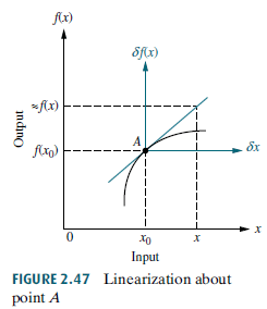
To obtain a linear mathematical model of a non-linear system it is necessary to suppose that the variable to be controlled only deviates very slightly from an operation point A of coordinates (xo, f (xo)), where xo is the input to the system and f (xo) is the output. At point A we can place a line with a certain slope and assume that for small changes δx around xo we have the output f (xo+δx) moving along this line, as shown in Figure 2-47:
We can use point A as a new center of coordinates where the independent variable δx corresponds to the input to the system, while the dependent variable δf (x) represents the output of the system. We make this convenient change of coordinates to use the equation of the slope ma of the line in the following way:
OrAnd so:
In the same way that:
The latter is a linear mathematical approximation for f (x).
This technique allows us to obtain a linear expression for f (x), around the point of operation A. Now, we are going to combine the obtained expressions for f (x) and δf (x). Another way of thinking it is to think that, around the point of operation A, f (x) has the value of f (xo) plus a small component of value maδx along a straight line of slope ma: Where (x-xo)is so small that it approaches δx. Mission accomplished, we will do this:
What theory allows us to do this? The Taylor series.
Taylor Series
The Taylor series are the expansion of a function f (x) in terms of the value of that function at a particular point xo, around that point and in terms of the derivatives of the function evaluated at that point:
When the excursion around the point xo is small, as the case that interests us, the derivatives of higher order can be ignored, so:
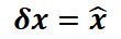
Knowing that the mx slope of a line at point xo is the derivative of the line evaluated in xo, we can adapt this last equation to our strategy and we obtain the formula that interests us: Where mx = df / dx evaluated at x = xo. Note that δx is now the independent variable, for which we use only a valid range of values around xo, so that δx is an excursion. Returning to Figure 2.47, this is the key tactic of the linearization process, we have created a coordinate system centered at point A, to replace the independent variable x with δx. We can continue using the δx notation or any other more practical notation such as: Let’s see how this works through examples.
Linearize a function
Suppose we have a system represented by the following function: Our task is to linearize f (x) around xo = π / 2. As: We find the following values and substitute them in the previous equation: Then we can represent our nonlinear system by means of the following negative line equation:
The result of the linearization of f (x) around xo = π / 2 can be seen in Figure 2.48:
Linearize a differential equation
Suppose now that our system is represented by the following differential equation: The presence of the term cosx makes the previous one a non-linear equation. It is requested to linearize said equation for small excursions around x = π / 4.
To replace the independent variable x with the excursion δx, we take advantage of the fact that: So:We proceed then to the substitution in the differential equation:We now apply the derivation rules:And for the term that involves the cosx function we apply the same methodology that we have just seen in the previous example for a given function, that is, linearize f (x) around xo = π / 4:
Note that in the previous equation the excursion is zero when the function is evaluated exactly at the point xo. The same happens when the slope is evaluated in xo:So:
Therefore, we can rewrite the differential equation in a linear fashion around the point xo =π /4 as follows:
That is to say:
Linearization of a system with two independent variables
The Taylor series enables us to work with functions or differential equations that have two independent variables. In this regard, the Taylor series applies the following formula:
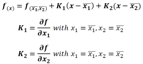
Where the point of operation has the coordinates ¯x1y ¯x2. For small excursions around the equilibrium point, we can obviate the higher order derivatives. The linear mathematical model for this nonlinear system around the point of operation is obtained from:
Example. Linearization of a system with two independent variables.
Linearization of magnetic sphere levitation system.
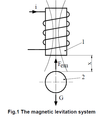
The magnetic suspension system of a sphere is shown in Figure 1.
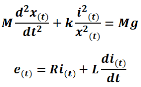
The objective of the system is to control the position of the steel sphere by adjusting the current in the electromagnet through the input voltage e(t). The dynamics of the system is represented by the following differential equations: Where:
It is requested to linearize the system around its equilibrium point.
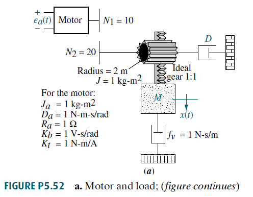
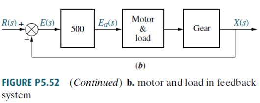
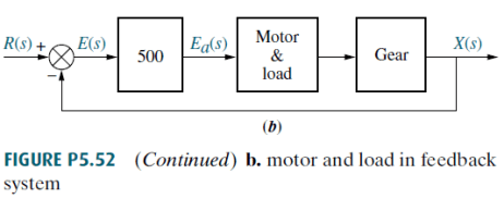
The mechanical system shown in Figure P5.52(a) is used as part of the unity feedback system shown in Figure P5.52(b). Find the values of M and D to yield 20% overshoot and 2 seconds settling time.
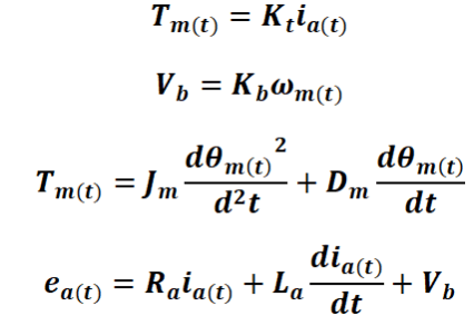
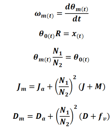
1. System Dynamic
where:
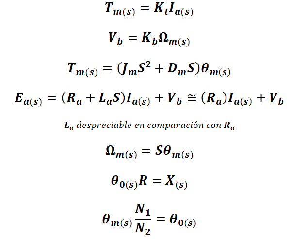
2. Laplace Transform
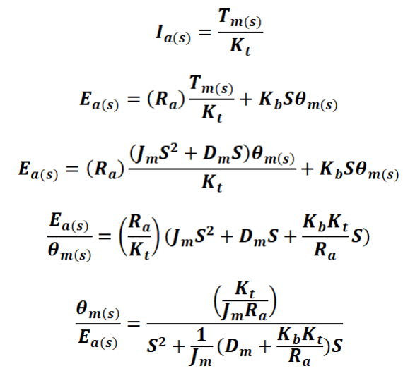
3. Motor&Load Transfer Function (θm(s)/Ea(s))
4. Direct Transfer Function
For the system:
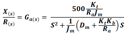
The open-loop transfer function Ga(s) is:
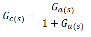
5. Closed-loop transfer function
The closed-loop transfer function Gc(s) is:
That is to say:
6. Calculation of M and D
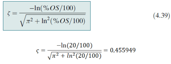
According to:
Besides:
In this way:
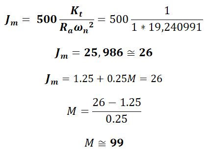
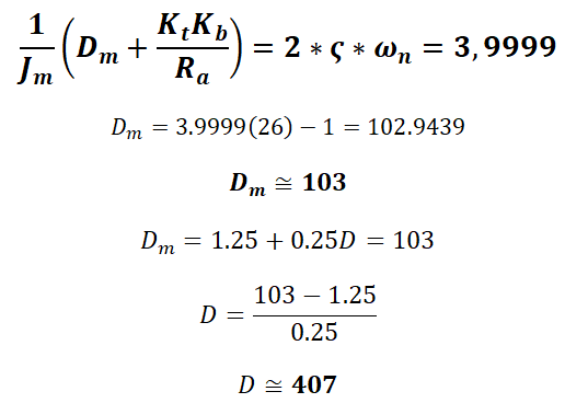
Meanwhile:
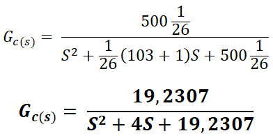
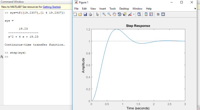
7. Matlab verification
We use Matlab to corroborate replacing all the values calculated in the original transfer function:
Find the values of M and D to yield 20% overshoot and 2 seconds settling time.
>> stepinfo (sys)
RiseTime: 0.3554
SettlingTime: 1.8989
SettlingMin: 0.9331
SettlingMax: 1.1999
Overshoot: 19.9890
Undershoot: 0
Peak: 1.1999
PeakTime: 0.8059
Written by Larry Francis Obando – Technical Specialist – Educational Content Writer
Mentoring Academic / Entrepreneur / Business
Copywriting, Content Marketing, White Papers (Spanish – English)
Escuela de Ingeniería Eléctrica de la Universidad Central de Venezuela, CCs.
Escuela de Ingeniería Electrónica de la Universidad Simón Bolívar, Valle de Sartenejas.
Escuela de Turismo de la Universidad Simón Bolívar, Núcleo Litoral.
Contact: Caracas, Quito, Guayaquil, Jaén, Villafranca de Ordizia- Telf. +34633129287
Find in generic terms, the transfer function of the unit feedback system shown in Figure P5.52 (b) of which the electromechanical system of Figure P5.52 (a) is a part.
1. System Dynamic
where:
2. Laplace Transform
3. Motor&Load Transfer Function (θm(s)/Ea(s))
4. Direct Transfer Function
For the system:
The open-loop transfer function Ga(s) is:
5. Closed-loop transfer function
The closed-loop transfer function Gc(s) is:
That is to say:
This problem is the first part of one where the transient response is requested so that the overshoot is 20% and the settling time is 2 seconds, see the complete problem in the following link: Example 1 – Transient response of an electromechanical system
Written by Larry Francis Obando – Technical Specialist – Educational Content Writer
Mentoring Academic / Entrepreneur / Business
Copywriting, Content Marketing, White Papers (Spanish – English)
Escuela de Ingeniería Eléctrica de la Universidad Central de Venezuela, CCs.
Escuela de Ingeniería Electrónica de la Universidad Simón Bolívar, Valle de Sartenejas.
Escuela de Turismo de la Universidad Simón Bolívar, Núcleo Litoral.
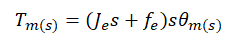
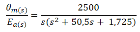
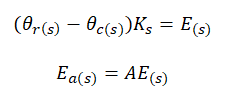
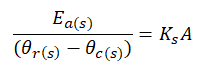
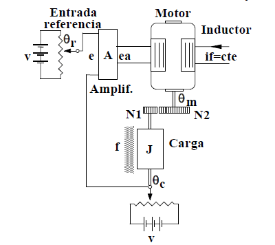
Obtain the mathematical model of the position control system of the figure. Get the block diagram and the ansfer function between the angle of the load and the reference angle θc(s)/θc(s).
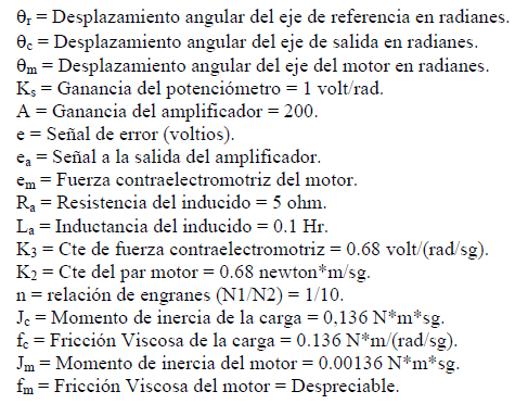
Data:
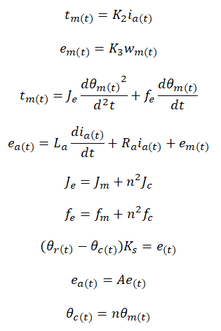
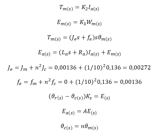
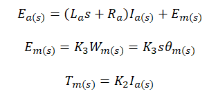
1. System dynamic
2. Laplace Transform
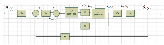
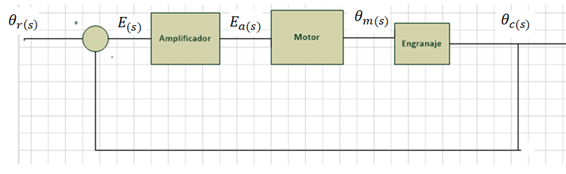
3. Block Diagram
Simplifying conveniently to obtain a model whose transfer function is known:
4. Transfer function of each block of the previous diagram.
Starting from:
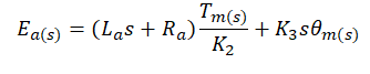
We obtain the following:Then, using:
and substituting, we obtain:
Substituting the value of the data in the previous equation, we obtain:
Simplifying:
On the other hand, the gain of the amplifier is obtained using:
From where:
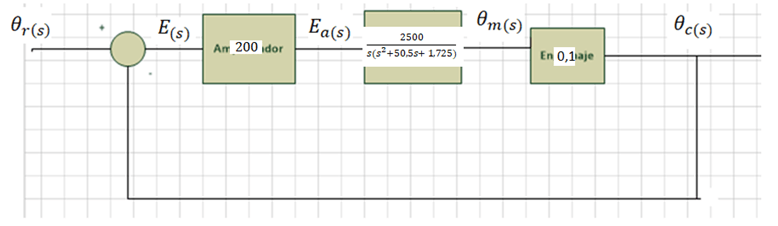
Finally, the gear constant is given by the data and is n = 1/10. We then obtain a block diagram with the following transfer functions:
5. System Transfer function.
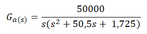
The open-loop transfer function Ga(s) of the system shown in the previous diagram is:
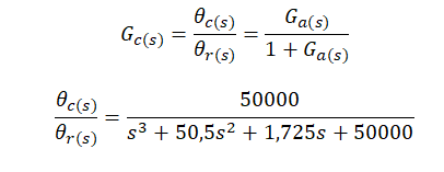
From where we can easily obtain the closed-loop transfer function Gc (s), which is what the statement asked, using the unit feedback:























 So:
So: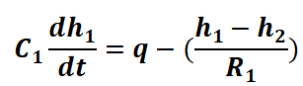 That is to say:
 In the other hand:
 That is:


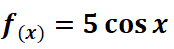 Our task is to linearize f (x) around xo = π / 2. As:
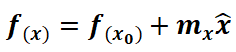 We find the following values and substitute them in the previous equation:
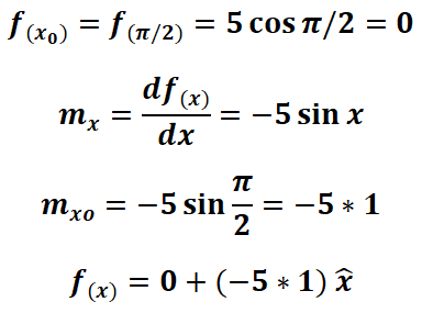 Then we can represent our nonlinear system by means of the following negative line equation: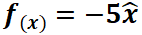
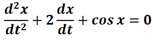 The presence of the term cosx makes the previous one a non-linear equation. It is requested to linearize said equation for small excursions around x = π / 4.
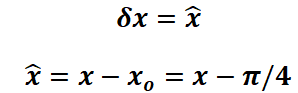 So:
So: We proceed then to the substitution in the differential equation:
 We now apply the derivation rules:
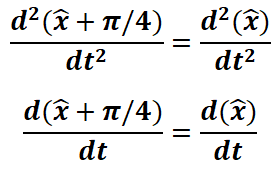 And for the term that involves the cosx function we apply the same methodology that we have just seen in the previous example for a given function, that is, linearize f (x) around xo = π / 4: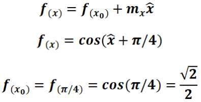
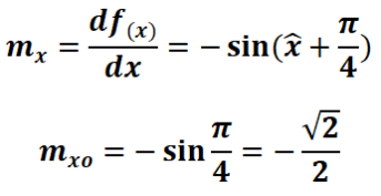 So:
So: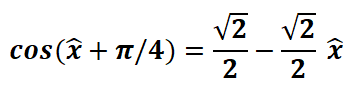
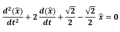
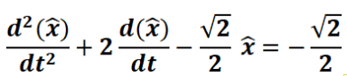
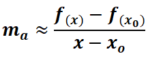
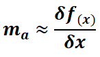 And so: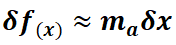

 Where (x-xo) is so small that it approaches δx. Mission accomplished, we will do this:

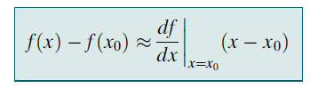
 Where mx = df / dx evaluated at x = xo. Note that δx is now the independent variable, for which we use only a valid range of values around xo, so that δx is an excursion. Returning to Figure 2.47, this is the key tactic of the linearization process, we have created a coordinate system centered at point A, to replace the independent variable x with δx. We can continue using the δx notation or any other more practical notation such as:
 Let’s see how this works through examples.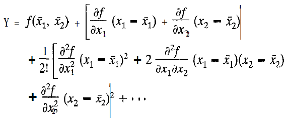
 Where: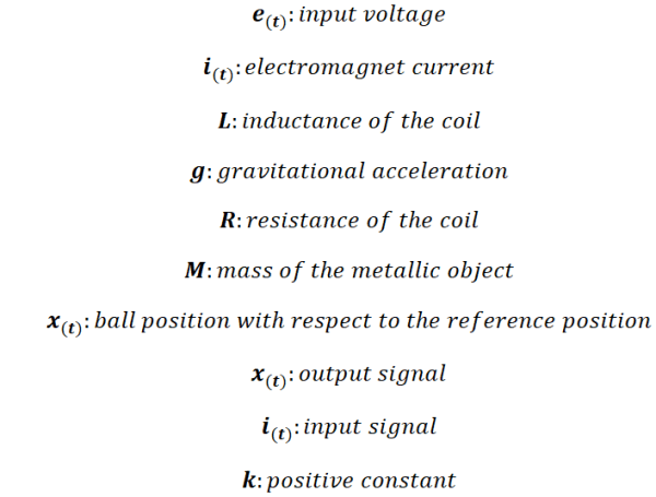
 That is to say: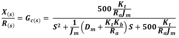
 We obtain the following:
 Then, using: