Sin categoría

The Discrete-Time Fourier Transform (DTFT)

When the system is linear and discrete time-invariant (LIT system), only one representation stands out as the most useful. It is called The Discrete-Time Fourier Transform (DTFT) and is based on the complex exponential signal set {ejωn}.

THE  DISCRETE-TIME FOURIER TRANSFORM (DTFT)

If x[n] is absolutely summable, that is:
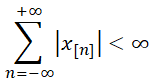
Then, the Discrete-Time Fourier Transform of x[n] is given by:
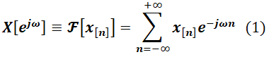
Example 1.

Determine the DTFT of x[n]:
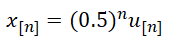
Solution.
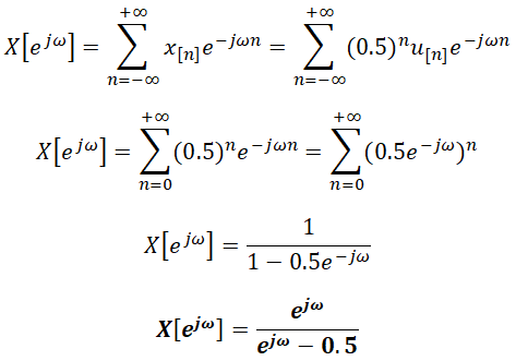
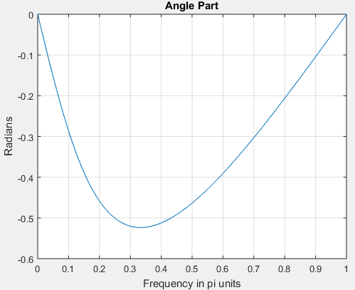
Since X[e] is a complex-valued function, will have to plots its magnitude and its angle (or the real part and imaginary part) with respect to ω separately to visually describe X[e]. Now ω is a real variable between –∞ and +, which would mean that we can plot only a part of the X[e] function. Using two important properties of the DTFT, we can reduce this domain to the [0,π] interval for real-valued sequences.

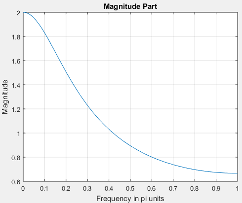
The following Matlab script allows us to plot every part of X(e) of example 1:

w=[0:1:500]*pi/500; X=exp(i*w)./(exp(i*w)-0.5*ones(1,501));
magX=abs(X);angX=angle(X);
plot(w/pi,magX); grid
xlabel(‘Frequency in pi units’); ylabel(‘Magnitude’);
title(‘Magnitude Part’)

This script yields:
w=[0:1:500]*pi/500; X=exp(i*w)./(exp(i*w)-0.5*ones(1,501));
angX=angle(X);
plot(w/pi,angX); grid
xlabel(‘Frequency in pi units’); ylabel(‘Radians’);
title(‘Angle Part’)

This script yields:
Example 2.

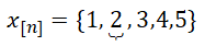
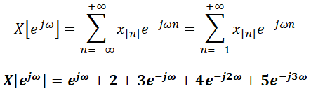
Determine the DTFT of the following finite-duration sequence:
Solution.
Two important properties

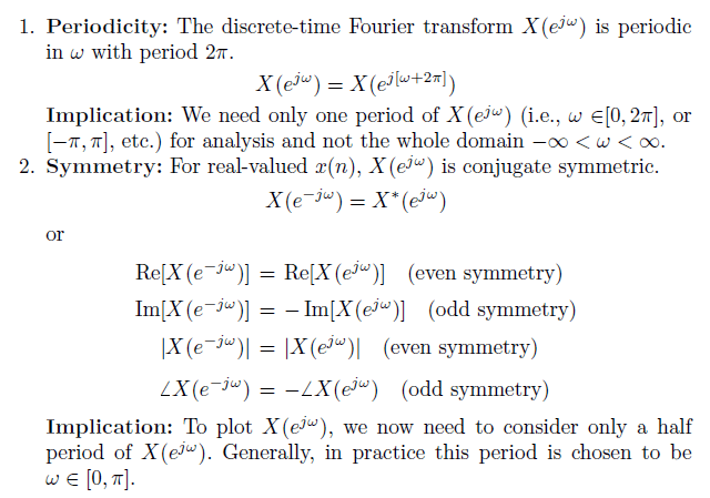
The following two properties are essential for DTFT analysis:
Some common DTFT Pairs

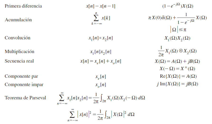
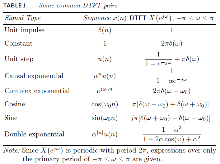
Derived from the previous properties, the DTFT of the following sequences, Table 1, are very useful:
Properties of the DTFT

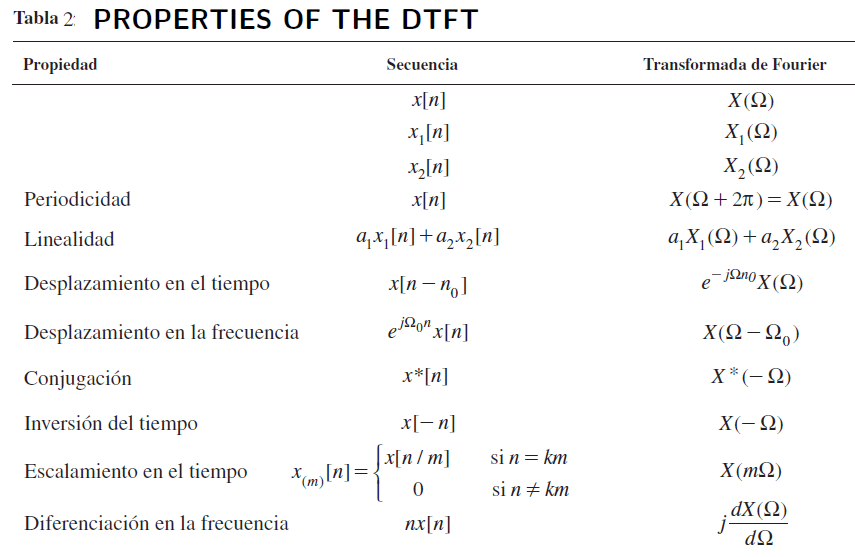
We now present the complete properties of the DTFT in Table 2:
These properties will be of remarkable value for the next application of the DTFT: The z-Transformation.

We early stated that the Fourier Transform representation is the most useful signal representation for LTI systems. That is true due to the following reason:

RESPONSE TO A COMPLEX EXPONENTIAL ejωon

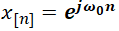
Let  be the input to an LTI system represented by the impulse response h[n]:
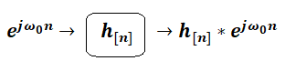
Then:
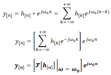
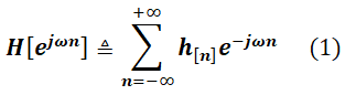
Definition: The FREQUENCY RESPONSE

FREQUENCY RESPONSE: The Discrete-Time Fourier Transform of an impulse response is called The Frequency Response (or The Transfer Function) of an LTI system and is denoted by:
In consequence, if x[n] is the input to an LTI system:
The system can be represented by:

and the output is as follows:

… Next: The Frequency Response of an LTI system

Source:

  • Digital Signal Processing Using Matlab, 3erd ed
  • Fundamentos_de_Señales_y_Sistemas_usando la Web y Matlab
  • Oppenheim – Señales y Sistemas
  • Análisis de Sistemas Lineales Asistido con Scilab – Un Enfoque desde la Ingeniería Eléctrica.

You can also be interested in:

Literature review by:

Prof. Larry Francis Obando – Technical Specialist – Educational Content Writer

Exercises are solved!!

WhatsApp:  +34633129287  Inmediate Attention!!

Twitter: @dademuch

Copywriting, Content Marketing, Tesis, Monografías, Paper Académicos, White Papers (Español – Inglés)

Escuela de Ingeniería Electrónica de la Universidad Simón Bolívar, USB Valle de Sartenejas.

Escuela de Ingeniería Eléctrica de la Universidad Central de Venezuela, UCV Caracas.

Escuela de Turismo de la Universidad Simón Bolívar, Núcleo Litoral.

Contacto: España. +34633129287

Caracas, Quito, Guayaquil, Jaén. 

WhatsApp:  +34633129287   

Twitter: @dademuch

FACEBOOK: DademuchConnection

email: dademuchconnection@gmail.com
Sin categoría

Filtros Digitales – Filtros FIR, IIR, AR, MA, ARMA – Procesamiento de señales

Filtro es un nombre genérico que se le da a un sistema lineal invariante en el tiempo (LTI por sus siglas en inglés) diseñado para un trabajo específico de selección de frecuencia o discriminación de frecuencia. Por lo tanto, los sistemas LTI de tiempo discreto también se denominan filtros digitales. Hay dos tipos de filtros digitales: filtros FIR y filtros IIR.

Introducción

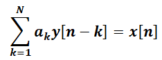
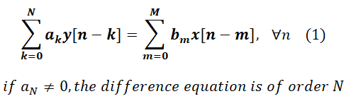
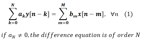
Un sistema discreto LTI también se puede describir mediante una ecuación en diferencias de coeficientes constantes lineales de la forma:

La imagen tiene un atributo ALT vacío; su nombre de archivo es image-75.png

Esta ecuación describe un enfoque recursivo para calcular la salida para la muestra n (o n muestras) dados los valores de entrada y los valores de salida calculados previamente. En la práctica, esta ecuación se calcula hacia adelante en el tiempo, desde n=-∞ a n=+∞. Por tanto, otra forma de escribir la ecuación (1) es:

La imagen tiene un atributo ALT vacío; su nombre de archivo es image-49.png
Filtro FIR 

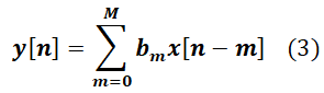
Si la respuesta al impulso unitario de un sistema LTI es de duración finita, el sistema se denomina filtro de respuesta de impulso de duración finita (o FIR: finite-duration impulse response). Por tanto, para un filtro FIR h[n]=0 para n<n1 y para n>n2. La siguiente parte de la ecuación de diferencia (2) describe un filtro FIR causal:

Además, h[0]=bo , h[1]=b1 ,… h[M]=bM. mientras que todos los demás h[n]’s valen 0. Los filtros FIR también se denominan filtros no recursivos o de promedio móvil (MA: non-recursive or moving average). En Matlab, los filtros FIR se representan como valores de respuesta de impulso {h[n]} o como coeficientes de ecuación de diferencia {bm} y {a0 =1}. Por lo tanto, para implementar filtros FIR en Matlab, podemos usar la función conv(x,h) o la función filter(b,1,x). Vea el siguiente ejemplo:

Ejemplo 1. 

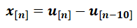
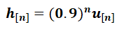
Let the following rectangular pulse x[n] be an input to an LTI system with impulse response h[n]:

Determine the output y[n] of the system.

Solution:

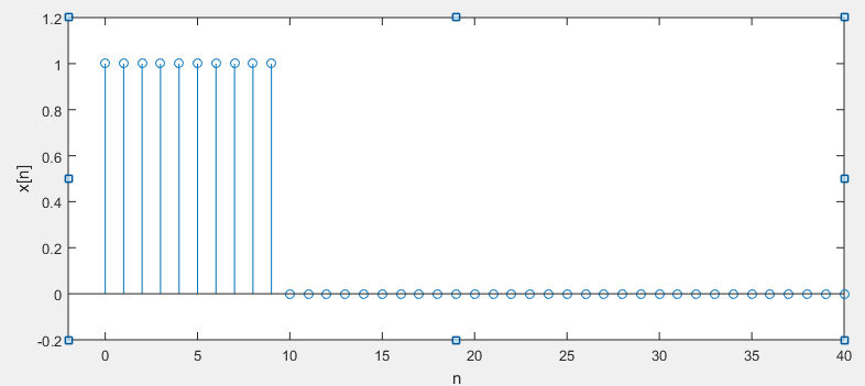
In Elementary sequences we have implemented the function stepseq for plotting the unit step function in discrete time, or any combination as example 1. Next Script allows plotting x[n].

n=[0:40];
x=stepseq(0,0,40)-stepseq(10,0,40);
stem(n,x)
xlabel(‘n’); ylabel(‘x[n]’)

Figure 1. Input sequence x[n], example 1.

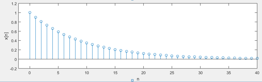
Next Script allows plotting h[n].

n=[0:40];
h=(0.9).^n;
stem(n,h)
xlabel(‘n’); ylabel(‘h[n]’)

Figure 2. Impulse response h[n] for system in example 1.

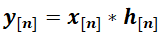
Now, we use conv Matlab function to determine y[n]:

y=conv(x,h);
n=[0:80];
stem(n,y);
xlabel(‘n’); ylabel(‘y[n]’)

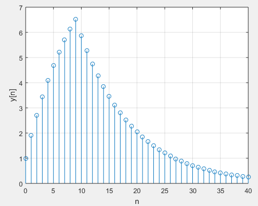
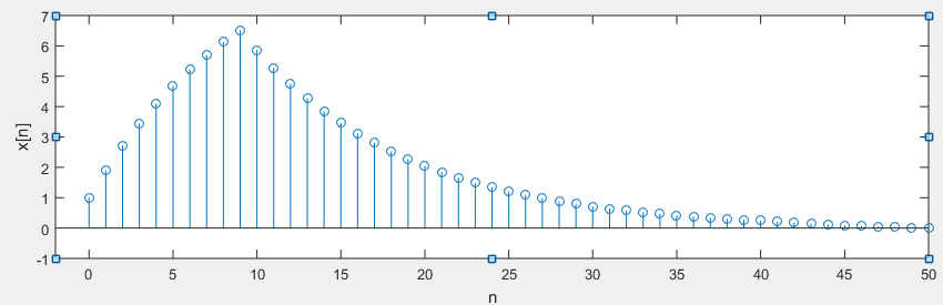
Figure 3. Output sequence y[n]=x[n]*h[n] for example 1.

Another approach is by using the filter function:

n=[0:40];
x=stepseq(0,0,40)-stepseq(10,0,40);
h=(0.9).^n;
y=filter(h,1,x);
stem(n,y)
xlabel(‘n’); ylabel(‘y[n]’)
grid

What yields:

Figure 4. Output sequence y[n]=x[n]*h[n] for example 1.

Hay una diferencia en los resultados de estas dos implementaciones que debe tenerse en cuenta. Como puede ver en la Figura 3, la secuencia de salida de la función conv(x,h) tiene una longitud mayor que las secuencias x[n] y h[n]. Por otro lado, la secuencia de salida de la función de filter(h,1,x) en la Figura 4 tiene exactamente la misma longitud que la secuencia de entrada x[n]. En la práctica, para la convolución de señales digitales se recomienda el uso de la función filter.

Cuidado: la función filter se puede utilizar para calcular la convolución indirectamente. Eso fue posible debido a que la respuesta al impulso en el ejemplo 1 era una secuencia exponencial infinita orientada a un lado para la cual podríamos determinar una representación de ecuación de diferencia. No todas las respuestas impulsionales de longitud infinita se pueden convertir en ecuaciones en diferencias.

IIR Filter

If the impulse response of an LTI system is of infinite duration, then the system is called an infinite-duration impulse response (or IIR) filter. The following part of the difference equation (2):

Si la respuesta al impulso de un sistema LTI es de duración infinita, entonces el sistema se denomina filtro de respuesta al impulso de duración infinita (o IIR: infinite-duration impulse response). Considere la siguiente parte de la ecuación en diferencias (2):

La ecuación previa describe un filtro recursivo en el que la salida y[n] se calcula de forma recursiva a partir de sus valores calculados previamente y se denomina filtro autorregresivo (AR: autoregressive). La respuesta al impulso de dicho filtro es de duración infinita y, por lo tanto, representa un filtro IIR. La ecuación general (2) también describe un filtro IIR. Tiene dos partes: una parte AR y una parte MA. Dicho filtro IIR se denomina promedio móvil autorregresivo o filtro ARMA. En Matlab, los filtros IIR se describen mediante los coeficientes de ecuación de diferencia {bm} y {ak} y se implementan mediante la función de filter(b,a,x). Vea el siguiente ejemplo:

Example 2

Given the following difference equation:

  1. Calculate and plot the impulse response h[n] at n=-20,…,100
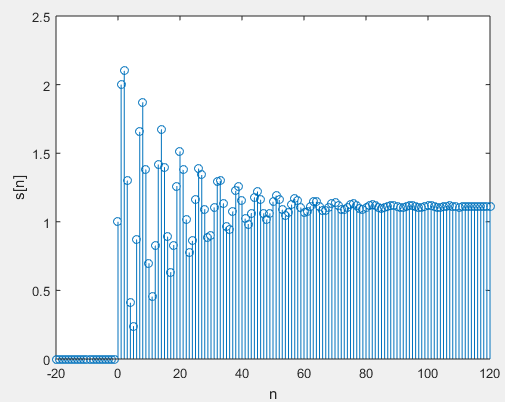
  2. Calculate and plot the unit step response s[n] at n=-20,…,100
  3. Is the system specified by h[n] stable?

Solution:

  1. To determine h[n] we use the following script:

n=[-20:120];
a=[1,-1,0.9];
b=[1];
h=impz(b,a,n);
stem(n,h)
grid
xlabel(‘n’); ylabel(‘h[n]’)

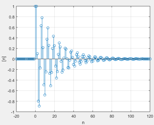
The script yields:

Figure 1. Impulse response h[n] for example 1.
  1. 2. To determine s[n] we use the following script:

n=[-20:120];
a=[1,-1,0.9];
b=[1];
x=stepseq(0,-20,120);
s=filter(b,a,x);
stem(n,s)
xlabel(‘n’); ylabel(‘s[n]’);

The script yields:

Figure 2. Step response s[n] for example 1.
  1. Is the system specified by h[n] stable?

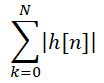
From Figure 1 we see that h[n] is practically zero n>120. Hence the sum:

Can be determined with the following script:

sum(abs(h))

This yields:

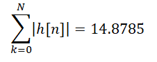
ans = 14.8785

That is to say:

This result implies that the system is stable. An alternate approach is to use the stability condition of the roots:

z=roots(a);
magz=abs(z)

magz =

0.9487
0.9487

Dado que la magnitud de ambas raíces es menor que uno, el sistema es estable.

En realidad, hay dos formas de resolver una ecuación en diferencias con coeficientes constantes lineales: encontrar la solución particular y la homogénea; encontrar las respuestas de entrada cero y de estado cero (the zero-input and the zero-state responses). Es mediante el uso de la transformada z que podemos derivar un método para obtener ambos.

Relacionado: Resolver ecuaciones diferenciales en tiempo discreto con Matlab

Fuentes:

  • Digital Signal Processing Using Matlab, 3erd ed
  • Fundamentos_de_Señales_y_Sistemas_usando la Web y Matlab
  • Oppenheim – Señales y Sistemas
  • Análisis de Sistemas Lineales Asistido con Scilab – Un Enfoque desde la Ingeniería Eléctrica.

Revisión literaria hecha por:

Prof. Larry Francis Obando – Technical Specialist – Educational Content Writer

Se hacen trabajos, se resuelven ejercicios!!

WhatsApp:  +34633129287  Atención Inmediata!!

Twitter: @dademuch

Copywriting, Content Marketing, Tesis, Monografías, Paper Académicos, White Papers (Español – Inglés)

Escuela de Ingeniería Electrónica de la Universidad Simón Bolívar, USB Valle de Sartenejas.

Escuela de Ingeniería Eléctrica de la Universidad Central de Venezuela, UCV Caracas.

Escuela de Turismo de la Universidad Simón Bolívar, Núcleo Litoral.

Contacto: España. +34633129287

Caracas, Quito, Guayaquil, Jaén. 

WhatsApp:  +34633129287   

Twitter: @dademuch

FACEBOOK: DademuchConnection

email: dademuchconnection@gmail.com

Sin categoría

Graficar el pulso rectangular en Matlab utilizando la transformada de Laplace

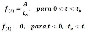
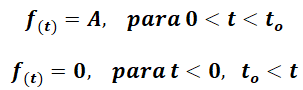
Considere la función pulso:

null

Donde A y t0 son constantes.

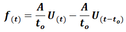
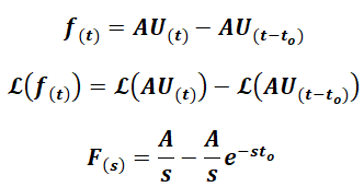
Esta función pulso puede considerarse una función escalón U(t) de altura A, que empieza en t=0, sobreimpuesta por un escalón U(t-to)  de altura –A, que empieza en  t=t0, es decir:

null

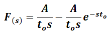
En este caso, la transformada de f(t) se obtiene mediante:

null

Aplicando la tabla para transformadas de Laplace (anexo) obtenemos:

null

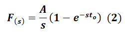
Por lo tanto, la transformada de Laplace la función pulso es:

null

Para el pulso rectangular, simplemente debemos considerar que:

null
Ejemplo 1. Gráfica en Matlab 

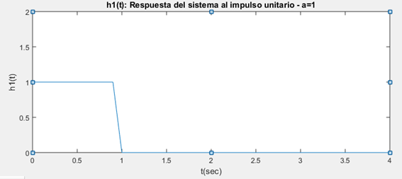
Suponga un pulso rectangular f(t) de altura A=1 y ancho t0=1. El siguiente script representa la forma más inmediata de graficar f(t) en Matlab (en este ejemplo f(t)=h1(t) es la respuesta al impulso unitario de un sistema cualquiera):

>> t=0:0.1:4;

>> h1=rectpuls(t,2);

>> plot(t,h1)

null

El script anterior utiliza el tiempo t para graficar la señal. Sin embargo, representar el pulso rectangular mediante la transformada de Laplace (representación en frecuencia) y utilizar dicha representación en Matlab, ofrece enormes ventajas para el análisis de sistemas lineales, y para la misma programación en Matlab, el cual ofrece un exuberante Control Toolbox para el caso en que una función está representada en frecuencia (como la función step, o la función impulse utilizada más tarde). Por ejemplo, la convolución entre dos señales en el dominio del tiempo, es un simple producto entre dos señales en el dominio de la frecuencia. Es por ello que procedemos de la siguiente manera.

La función pulso rectangular f(t) de ancho t0 puede considerarse una función escalón U(t) de altura A, que empieza en t=0, y es luego anulada (no sobreimpuesta como el caso anterior) por un escalón U(t-to)  de altura –A, que empieza en  t=t0, es decir:

null

Por lo tanto, la transformada de Laplace la función pulso rectangular es:

null
Ejemplo 2. Gráfica en Matlab 

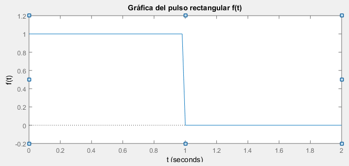
Suponga el pulso rectangular f(t) de altura A=1 y ancho t0=1 del ejemplo 1. El siguiente script utiliza la transformada de Laplace la función pulso rectangular en combinación con la respuesta al impulso de un sistema cualquiera, para graficar el pulso rectangular:

s=tf(‘s’);
f1=tf([1],[1 0]);
f2=exp(-s)*tf([1],[1 0]);
f=f1-f2;
impulse(f)
xlabel(‘t’); ylabel(‘f(t)’)
title(‘Gráfica del pulso rectangular f(t)’)

Es de gran valor recordar que la respuesta al impulso en el dominio de la frecuencia nos permite obtener de manera inmediata la Función de Transferencia del sistema.

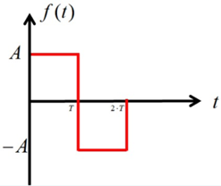
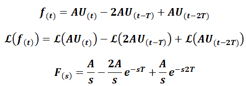
Con la ecuación (2) en la mano podemos adaptar este resultado a situaciones particulares. Suponga el caso de un pulso rectangular como el mostrado en la siguiente Figura:

null

Al aplicar el mismo procedimiento vemos que:

null

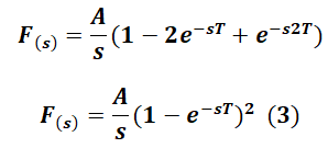
Por lo tanto, la transformada de Laplace la función de la Figura es como en la ecuación (3):

null
Gráfica en Matlab 

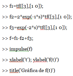
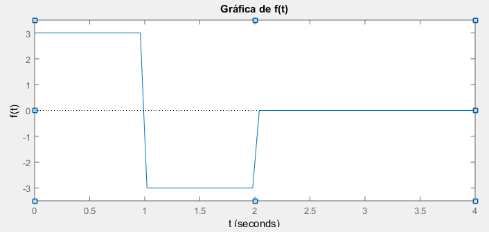
En la ecuación anterior considere T=1, A=3. Es decir, dos pulsos rectangulares de ancho 1 y amplitud 3, que inicia en t=0. El siguiente script permite obtener la gráfica de f(t) en Matlab:

La imagen tiene un atributo ALT vacío; su nombre de archivo es image-9.png

Ejemplo 3.

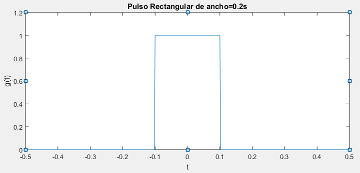
El siguiente código simula un pulso rectangular con un ancho de pulso deseado y el gráfico resultante:

fs=500; %sampling frequency
T=0.2; %width of the rectangular pulse in seconds
t=0.5:1/fs:0.5; %time base
g=(t>-T/2).(t(t==T/2)+0.5(t==-T/2); g=(t>-T/2).(t<T/2)+0.5(t==T/2)+0.5(t==-T/2); %rectpuls(t,T); %using inbuilt function (signal proc toolbox)
plot(t,g); title([‘Pulso Rectangular de ancho=’,num2str(T),’s’])

Pulso Rectangular de ancho 0.2 segundos.

Referencia:

  • Ingeniería de control moderna (Ogata)

Otros temas de interes:

Revisión literaria hecha por:

Prof. Larry Francis Obando – Technical Specialist – Educational Content Writer

Se hacen trabajos, se resuelven ejercicios!!

WhatsApp:  +34633129287  Atención Inmediata!!

Twitter: @dademuch

Copywriting, Content Marketing, Tesis, Monografías, Paper Académicos, White Papers (Español – Inglés)

Escuela de Ingeniería Electrónica de la Universidad Simón Bolívar, USB Valle de Sartenejas.

Escuela de Ingeniería Eléctrica de la Universidad Central de Venezuela, UCV CCs

Escuela de Turismo de la Universidad Simón Bolívar, Núcleo Litoral.

Contacto: Caracas, Quito, Guayaquil, Jaén. +34633129287

WhatsApp:  +34633129287   

Twitter: @dademuch

FACEBOOK: DademuchConnection

email: dademuchconnection@gmail.com
Sin categoría

Autofunciones de sistemas LTI analógicos

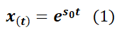
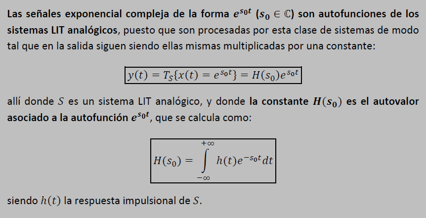
Sea S un sistema LTI (lineal e invariante en el tiempo) analógico cualquier y sea h(t) su respuesta impulsiva. Considérese que la señal de entrada de S es una señal exponencial compleja de la forma siguiente:

Allí donde s0 es una constante compleja (s complejos)

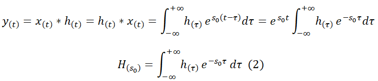
Al calcular la señal de salida de S como resultado de la convolución entre x(t)  y h(t), se observa lo siguiente:

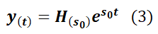
En consecuencia:

Allí donde, independientemente de si h(t) es una señal real o compleja, H(s0)  es un valor constante (no depende de t) y, en general, complejo (puesto que s0 complejos).

Así pues se observa que la salida de un sistema LTI analógico cualquier ante cualquier señal exponencial compleja de la forma expresada en la ecuación (1) es igual a esa misma señal exponencial compleja multiplicada por una constante. En concreto, por la señal denominada en la ecuación (2). Se observa además que dicha constante depende únicamente de h(t) (la respuesta impulsiva del sistema) y del valor de s0.

En este punto enunciamos el teorema de las autofunciones de los sistemas LTI analógicos:

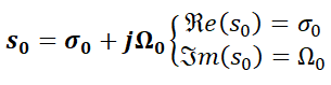
En primer lugar conviene notar que la constante s0 tiene parte real y parte imaginaria:

Por lo tanto, vemos que las autofunciones de los sistema LTI analógicos pueden ser vistas como el resultado del producto de una señal exponencial real y una señal exponencial compleja:

Allí donde,  σ0 y Ω0 son constantes reales (σ0 y Ω0 )

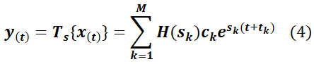
Y en segundo lugar, puesto que todo sistema LTI es, por definición, lineal e invariante en el tiempo, ya podemos extraer la consecuencia más inmediata, pero de enorme importancia, del teorema de las autofunciones. Sea una combinación lineal arbitraria de M exponenciales complejas:

La salida de cualquier sistema LTI analógico S ante una entrada de la forma expresada en la ecuación anterior, es otra combinación lineal de las mismas exponenciales complejas:

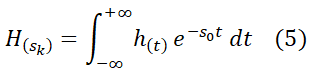
Donde H(sk) se calcula a partir de h(t), la respuesta impulsiva de S, del siguiente modo:

A continuación se ilustra la utilidad práctica de las autofunciones.

Ejemplo 1

Sea S un sistema LTI analógico y sea h(t) su respuesta impulsiva:

Se pide calcular la salida del sistema S ante la siguiente señal de entrada:

Respuesta:

Para aplicar el teorema de autofunciones expresamos como una combinación lineal de exponenciales complejas:

Aplicando la ecuación (4), la salida es la siguiente:

Procedemos a calcular cada uno de los factores H(i):

Por otra parte:

Además:

Por lo tanto:

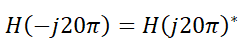
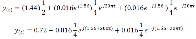
Finalmente la expresión definitiva para y(t) es:

En consecuencia:

Fuentes:

  1. Fundamentos_de_Señales_y_Sistemas_usando la Web y Matlab
  2. Oppenheim – Señales y Sistemas
  3. Análisis de Sistemas Lineales Asistido con Scilab – Un Enfoque desde la Ingeniería Eléctrica.
  4. Amplificador Operacional
  5. CIRCUITO TRANSFORMADO DE LAPLACE
  6. DINAMICA CIRCUITOS
  7. INTRODUCCION A LAS SENALES Y SISTEMAS
  8. RESPUESTA EN FRECUENCIA
  9. TRANSFORMACION DE LAPLACE
  10. Control Systems Engineering, Nise
  11. Convolución LTI

Te puede interesar:

Escrito por Prof. Larry Francis Obando – Technical Specialist – Educational Content Writer – Twitter: @dademuch

Se hacen trabajos, se resuelven ejercicios!!

WhatsApp:  +34633129287  Atención Inmediata!!

Mentoring Académico / Emprendedores / Empresarial

Copywriting, Content Marketing, Tesis, Monografías, Paper Académicos, White Papers (Español – Inglés)

Escuela de Ingeniería Electrónica de la Universidad Simón Bolívar, USB Valle de Sartenejas.

Escuela de Ingeniería Eléctrica de la Universidad Central de Venezuela, UCV CCs

Escuela de Turismo de la Universidad Simón Bolívar, Núcleo Litoral.

Contacto:  Caracas, Quito, Guayaquil, España: Tlf. +34633129287.

WhatsApp: +34 633129287

Twitter: @dademuch

FACEBOOK: DademuchConnection

email: dademuchconnection@gmail.com
Sin categoría

Digital Filters – FIR and IIR Filters – MA Filters – Examples

Filter is a generic name that means a linear time-invariant system designed for a specific job of frequency selection or frequency discrimination. Hence discrete-time LTI systems are also called digital filters. There are two types of digital filters: FIR Filters and IIR Filters.

Preliminaries

An LTI discrete system can also be described by a linear constant coefficient difference equation of the form:

La imagen tiene un atributo ALT vacío; su nombre de archivo es image-75.png

This equation describes a recursive approach for computing the current output, given the input values and previously computed output values. In practice, this equation is computed forward in time, from n=-∞ to n=+∞. Therefore, another form of equation (1) is:

La imagen tiene un atributo ALT vacío; su nombre de archivo es image-49.png
FIR Filter

If the unit impulse response of an LTI system is of finite duration, the system is called a finite-duration impulse response (or FIR) filter.  Hence for a FIR filter h[n]=0 for n<n1 and for n>n2. The following part of the difference equation (2) describes a causal FIR filter:

Furthermore, h[0]=bo , h[1]=b1 ,… h[M]=bM . while all the other h[n]’s are 0. FIR filters are also called non-recursive or moving average (MA) filters. In Matlab FIR filters are represented either as impulse response values {h[n]} or as difference equation coefficients {bm} and {a0 =1}. Therefore, to implement FIR filters in Matlab, we can use either the conv(x,h) function, or the filter(b,1,x) function. See the following example:

Example 1. 

Let the following rectangular pulse x[n] be an input to an LTI system with impulse response h[n]:

Determine the output y[n] of the system.

Solution:

In Elementary sequences we have implemented the function stepseq for plotting the unit step function in discrete time, or any combination as example 1. Next Script allows plotting x[n].

n=[0:40];
x=stepseq(0,0,40)-stepseq(10,0,40);
stem(n,x)
xlabel(‘n’); ylabel(‘x[n]’)

Figure 1. Input sequence x[n], example 1.

Next Script allows plotting h[n].

n=[0:40];
h=(0.9).^n;
stem(n,h)
xlabel(‘n’); ylabel(‘h[n]’)

Figure 2. Impulse response h[n] for system in example 1.

Now, we use conv Matlab function to determine y[n]:

y=conv(x,h);
n=[0:80];
stem(n,y);
xlabel(‘n’); ylabel(‘y[n]’)

Figure 3. Output sequence y[n]=x[n]*h[n] for example 1.

Another approach is by using the filter function:

n=[0:40];
x=stepseq(0,0,40)-stepseq(10,0,40);
h=(0.9).^n;
y=filter(h,1,x);
stem(n,y)
xlabel(‘n’); ylabel(‘y[n]’)
grid

What yields:

Figure 4. Output sequence y[n]=x[n]*h[n] for example 1.

There is a difference in the outputs of these two implementations that should be noted. As you can see in Figure 3, the output sequence from conv(x,h) function has a longer length than both x[n] and h[n] sequences. On the other hand, the output sequence from the filter(h,1,x) function in Figure 4 has exactly the same length as the input x[n] sequence. In practice, the use of the filter function is encouraged.

Watch out: The filter function can be used to compute the convolution indirectly. That was possible because of the impulse response in example 1 was a one-side exponential sequence for wich we could determine a difference equation representation. Not all infinite-lenght impulse responses can be converted into difference equations.

IIR Filter

If the impulse response of an LTI system is of infinite duration, then the system is called an infinite-duration impulse response (or IIR) filter. The following part of the difference equation (2):

Describes a recursive filter in which the output y[n] is recursively computed from its previously computed values and is called an autoregressive (AR) filter. The impulse response of such filter is of infinite duration and hence it represents and IIR filter. The general equation (2) also describes an IIR filter. It has two parts: an AR part and a MA part. Such an IIR filter is called an autoregressive moving average, or an ARMA filter. In Matlab, IIR filters are described by the difference equation coefficients {bm} and {ak} and are implemented by the filter(b,a,x) function. See the following example:

Example 2

Given the following difference equation:

  1. Calculate and plot the impulse response h[n] at n=-20,…,100
  2. Calculate and plot the unit step response s[n] at n=-20,…,100
  3. Is the system specified by h[n] stable?

Solution:

  1. To determine h[n] we use the following script:

n=[-20:120];
a=[1,-1,0.9];
b=[1];
h=impz(b,a,n);
stem(n,h)
grid
xlabel(‘n’); ylabel(‘h[n]’)

The script yields:

Figure 1. Impulse response h[n] for example 1.
  1. 2. To determine s[n] we use the following script:

n=[-20:120];
a=[1,-1,0.9];
b=[1];
x=stepseq(0,-20,120);
s=filter(b,a,x);
stem(n,s)
xlabel(‘n’); ylabel(‘s[n]’);

The script yields:

Figure 2. Step response s[n] for example 1.
  1. Is the system specified by h[n] stable?

From Figure 1 we see that h[n] is practically zero n>120. Hence the sum:

Can be determined with the following script:

sum(abs(h))

This yields:

ans = 14.8785

That is to say:

This result implies that the system is stable. An alternate approach is to use the stability condition of the roots:

z=roots(a);
magz=abs(z)

magz =

0.9487
0.9487

Since the magnitude of both roots are less than one, the system is stable.

Actually, there are two forms of solving a linear constant coefficient difference equation: finding the particular and the homogeneous solutions; finding the zero-input and the zero-state responses. It is by using the z-transform that we can derive a method to obtain both.

Related: Solving discrete-time differential equations with Matlab

Source:

  • Digital Signal Processing Using Matlab, 3erd ed
  • Fundamentos_de_Señales_y_Sistemas_usando la Web y Matlab
  • Oppenheim – Señales y Sistemas
  • Análisis de Sistemas Lineales Asistido con Scilab – Un Enfoque desde la Ingeniería Eléctrica.

You can also be interested in:

Literature review by:

Prof. Larry Francis Obando – Technical Specialist – Educational Content Writer

Exercises are solved!!

WhatsApp:  +34633129287  Inmediate Attention!!

Twitter: @dademuch

Copywriting, Content Marketing, Tesis, Monografías, Paper Académicos, White Papers (Español – Inglés)

Escuela de Ingeniería Electrónica de la Universidad Simón Bolívar, USB Valle de Sartenejas.

Escuela de Ingeniería Eléctrica de la Universidad Central de Venezuela, UCV Caracas.

Escuela de Turismo de la Universidad Simón Bolívar, Núcleo Litoral.

Contacto: España. +34633129287

Caracas, Quito, Guayaquil, Jaén. 

WhatsApp:  +34633129287   

Twitter: @dademuch

FACEBOOK: DademuchConnection

email: dademuchconnection@gmail.com
Sin categoría

Resolver ecuaciones diferenciales en tiempo discreto con Matlab

Un sistema LTI (lineal e invariante en el tiempo) de tiempo discreto puede ser descrito mediante una ecuación diferencial lineal (ó ecuación lineal en diferencias) con coeficientes constantes de la forma:

La ecuación (1) describe un método recursivo para calcular la salida y[n], dado los valores de la entrada x[n] y valores previos de la misma salida y[n]. En la práctica, esta ecuación se calcula hacia adelante en el tiempo, de n=-∞ a n=∞. En consecuencia, otra forma de escribir esta ecuación es:

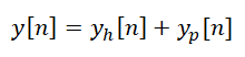
Una solución para la ecuación (2) puede ser obtenida de la forma:

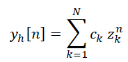
La parte homogénea yh[n] está dada por:

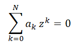
Donde zk, k=1,…,N son N raíces (también conocidas como frecuencias naturales) de la ecuación característica:

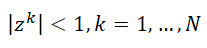
La ecuación característica es importante porque determina la estabilidad del sistema. Si las raíces zk satisfacen la siguiente condición:

Entonces el sistema causal de la ecuación (2) es estable. La solución particular, yp[n], está determinada por la parte derecha de la ecuación (1), para lo cual utilizaremos la transformada z (z-transform) en la determinación de la solución de una ecuación en diferencias.

Matlab solving

Una función llamada filter está disponible en Matlab para resolver Discrete-Time difference equations, dados los valores de la entrada y los coeficientes de la ecuación en diferencias. En su forma más simple la función es invocada por:

y=filter(b,a,x)

Donde b y a son las matrices de los coeficientes de la ecuación (1), y x es la matriz de la secuencia de entrada. Debemos asegurarnos de que el coeficiente a0 no sea igual a cero.

Para determinar y graficar la respuesta al impulso, Matlab además provee la función impz:

h=impz(b,a,n);

Calcula muestras de la respuesta al impulso del filtro en los índices de muestra dados en n con coeficientes de numerador en b y coeficientes de denominador en a.

Ejemplo 1.

Dada la siguiente ecuación en diferencias:

  1. Calculate and plot the impulse response h[n] at n=-20,…,100
  2. Calculate and plot the unit step response s[n] at n=-20,…,100
  3. Is the system specified by h[n] stable?

Solution:

  1. To determine h[n] we use the following script:

n=[-20:120];
a=[1,-1,0.9];
b=[1];
h=impz(b,a,n);
stem(n,h)
grid
xlabel(‘n’); ylabel(‘h[n]’)

The script yields:

Figure 1. Impulse response h[n] for example 1.
  1. 2. To determine s[n] we use the following script:

n=[-20:120];
a=[1,-1,0.9];
b=[1];
x=stepseq(0,-20,120);
s=filter(b,a,x);
stem(n,s)
xlabel(‘n’); ylabel(‘s[n]’);

The script yields:

Figure 2. Step response s[n] for example 1.
  1. Is the system specified by h[n] stable?

From Figure 1 we see that h[n] is practically zero n>120. Hence the sum:

Can be determined with the following script:

sum(abs(h))

This yields:

ans = 14.8785

That is to say:

This result implies that the system is stable. An alternate approach is to use the stability condition of the roots:

z=roots(a);
magz=abs(z)

magz =

0.9487
0.9487

Since the magnitude of both roots are less than one, the system is stable.

Puede estar interesado también en:

Revisión literaria hecha por:

Prof. Larry Francis Obando – Technical Specialist – Educational Content Writer

Se hacen trabajos, se resuelven ejercicios!!

WhatsApp:  +34633129287  Atención Inmediata!!

Twitter: @dademuch

Copywriting, Content Marketing, Tesis, Monografías, Paper Académicos, White Papers (Español – Inglés)

Escuela de Ingeniería Electrónica de la Universidad Simón Bolívar, USB Valle de Sartenejas.

Escuela de Ingeniería Eléctrica de la Universidad Central de Venezuela, UCV CCs

Escuela de Turismo de la Universidad Simón Bolívar, Núcleo Litoral.

Contacto: España. +34633129287

Caracas, Quito, Guayaquil, Jaén. 

WhatsApp:  +34633129287     

Twitter: @dademuch

FACEBOOK: DademuchConnection

email: dademuchconnection@gmail.com
Sin categoría

Solving discrete-time differential equations with Matlab

An LTI discrete system can also be described by a linear constant coefficient difference equation of the form:

This equation describes a recursive approach for computing the current output, given the input values and previously computed output values. In practice, this equation is computed forward in time, from n=-∞ to n=∞. Therefore, another form of this equation is:

A solution to equation (2) can be obtained in the form:

The homogeneous part yh[n] is given by:

Where zk, k=1,…,N are N roots (also called natural frequencies) of the characteristic equation:

This characteristic equation is important in determining the stability of the system. If roots zk satisfy the condition:

Then a casual system described by equation (2) is stable. The particular part of the solution, yp[n], is determined from the right-hand side of equation (1), where we will use z-transform for solving the difference equation.

Matlab solving

A function called filter in available in Matlab to solve Discrete-Time difference equations, given the input and the difference equation coefficients. In its simplest form it is invoked by:

y=filter(b,a,x)

Where b and a are the coefficient arrays from the equation (1), and x is the input sequence array. One must ensure that the coefficient a0 not be zero.

To compute and plot impulse response, Matlab also provides the function impz:

h=impz(b,a,n);

It computes samples of the impulse response of the filter at the sample indices given in n with numerator coefficients in b and denominator coefficients in a.

Example 1.

Given the following difference equation:

  1. Calculate and plot the impulse response h[n] at n=-20,…,100
  2. Calculate and plot the unit step response s[n] at n=-20,…,100
  3. Is the system specified by h[n] stable?

Solution:

  1. To determine h[n] we use the following script:

n=[-20:120];
a=[1,-1,0.9];
b=[1];
h=impz(b,a,n);
stem(n,h)
grid
xlabel(‘n’); ylabel(‘h[n]’)

The script yields:

Figure 1. Impulse response h[n] for example 1.
  1. 2. To determine s[n] we use the following script:

n=[-20:120];
a=[1,-1,0.9];
b=[1];
x=stepseq(0,-20,120);
s=filter(b,a,x);
stem(n,s)
xlabel(‘n’); ylabel(‘s[n]’);

The script yields:

Figure 2. Step response s[n] for example 1.
  1. Is the system specified by h[n] stable?

From Figure 1 we see that h[n] is practically zero n>120. Hence the sum:

Can be determined with the following script:

sum(abs(h))

This yields:

ans = 14.8785

That is to say:

This result implies that the system is stable. An alternate approach is to use the stability condition of the roots:

z=roots(a);
magz=abs(z)

magz =

0.9487
0.9487

Since the magnitude of both roots are less than one, the system is stable.

Actually, there are two forms of solving a linear constant coefficient difference equation: finding the particular and the homogeneous solutions; finding the zero-input and the zero-state responses. It is by using the z-transform that we can derive a method to obtain both.

Finding the particular and the homogeneous solutions

In construction…

Working with initial conditions – The zero-input and the zero-state responses.

In Matlab another form of the function filter can be used to solve for the differential equation, given its initial conditions.

In construction…

Related: Digital Filters – Moving Average Filters

You could be also interested in:

Source:

  • Digital Signal Processing Using Matlab, 3erd ed
  • Fundamentos_de_Señales_y_Sistemas_usando la Web y Matlab
  • Oppenheim – Señales y Sistemas
  • Análisis de Sistemas Lineales Asistido con Scilab – Un Enfoque desde la Ingeniería Eléctrica.

Literature review by:

Prof. Larry Francis Obando – Technical Specialist – Educational Content Writer

Exercises are solved!!

WhatsApp:  +34633129287  Inmediate Attention!!

Twitter: @dademuch

Copywriting, Content Marketing, Tesis, Monografías, Paper Académicos, White Papers (Español – Inglés)

Escuela de Ingeniería Electrónica de la Universidad Simón Bolívar, USB Valle de Sartenejas.

Escuela de Ingeniería Eléctrica de la Universidad Central de Venezuela, UCV Caracas.

Escuela de Turismo de la Universidad Simón Bolívar, Núcleo Litoral.

Contacto: España. +34633129287

Caracas, Quito, Guayaquil, Jaén. 

WhatsApp:  +34633129287   

Twitter: @dademuch

FACEBOOK: DademuchConnection

email: dademuchconnection@gmail.com
Sin categoría

La función coseno en tiempo discreto – Matlab

Las señales sinusoidales son muy importantes porque la Transformada de Fourier afirma que la mayoría de las señales de uso práctico se pueden descomponer en una suma infinita de señales sinusoidales. Una señal sinusoidal en el tiempo discreto se representa mediante:

Donde A es la amplitud y θo es la fase en radianes. Por su parte, ωo=2πf es la frecuencia angular y x[n] puede ser escrita como:

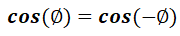
Es muy importante entender que la frecuencia de una sinusoide de tiempo discreto no está definida de forma única. Esta ambigüedad fundamental se debe a la siguiente propiedad trigonométrica:

En palabras, el valor de una sinusoide no cambia si un número entero múltiplo de se suma a su argumento. Sumando 2πkn al argumento de la ecuación (1) obtenemos:

Se distinguen dos casos. Si k≥-f, la ecuación (2) es equivalente a una sinusoide con frecuencia f+k sin cambio de fase:

Por otra parte, si k<-f, la ecuación (3) conduce a una frecuencia negativa. Para evita esto, definimos:

Además hacemos uso de la siguiente propiedad:

En consecuencia, volviendo a las ecuaciones (2) y (3), obtenemos una sinusoide de frecuencia l-f con una inversión de fase:

En conclusión: «a discrete-time sinusoid with frequency f is identical to a same-phase sinusoid of frequency f+k, where k is any integer greater than –f, or to a phase-reversed sinusoid of frequency l-f if l>f«.

La ecuación (3) se puede expresar de forma más concisa utilizando la notación exponencial compleja:

Because value of a complex exponential does not change if a multiple of is added to its argument, we get:

Equation (5) is equivalent to equation (4). Because of this fundamental frequency ambiguity, we will often implicitly assume that the angular frequency of a discrete-time sinusoid is restricted to the range –π≤ω≤π, or equivalent, that -1/2≤f≤1/2.

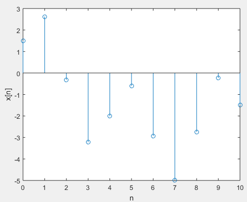
The Matlab function cos or sin generates the sinusoidal sequences. For example, for x[n]=3cos(0.1πn+π/3)+2sin(0.5πn), 0n10, we will use the following script:

n=[0:10]; x=3*cos(0.1*pi*n+pi/3)+2*sin(0.5*pi*n);
stem(n,x)

This script yields:

Source:

  • Digital Signal Processing Using Matlab, 3erd ed

PREVIOUS:

Literature review by:

Prof. Larry Francis Obando – Technical Specialist – Educational Content Writer

Exercises are solved!!

WhatsApp:  +34633129287  Inmediate Attention!!

Twitter: @dademuch

Copywriting, Content Marketing, Tesis, Monografías, Paper Académicos, White Papers (Español – Inglés)

Escuela de Ingeniería Electrónica de la Universidad Simón Bolívar, USB Valle de Sartenejas.

Escuela de Ingeniería Eléctrica de la Universidad Central de Venezuela, UCV CCs

Escuela de Turismo de la Universidad Simón Bolívar, Núcleo Litoral.

Contacto: España. +34633129287

Caracas, Quito, Guayaquil, Jaén. 

WhatsApp:  +34633129287     

Twitter: @dademuch

FACEBOOK: DademuchConnection

email: dademuchconnection@gmail.com
Sin categoría

The sinusoidal function in discrete time – Matlab

Sine waves are important because Fourier´s Theorem states that most signals of practical interest can be decomposed into an infinite sum of sine waves. Discrete-time signals (also called time series) are defined over the set of integers, that is, they are indexed sequences. A discrete-time sine wave is defined by:

Where A is an amplitude and  θo is the phase in radians. Meanwhile, ωo=2πf is the angular frequency and x[n] could be written as:

It is important to understand that the frequency of a discrete-time sinusoid is not uniquely defined. This fundamental ambiguity is a consequence of a basic trigonometric property:

In words, the value of a sinusoid does not change if an integer multiple of is added to its argument. Adding the 2πkn to the argument of equation (1) we get:

Two cases must be distinguished. If k≥-f, the equation (2) is equivalent to a sinusoid with frequency f+k with no change in phase:

On the other hand, if k<-f, equation (3) leads to a negative frequency. To avoid this, we introduce:

We also make use of the property:

In consequence, returning to equations (2) and (3), we obtain a sinusoid of frequency l-f with a reversal in phase:

In conclusion, a discrete-time sinusoid with frequency f is identical to a same-phase sinusoid of frequency f+k, where k is any integer greater than –f, or to a phase-reversed sinusoid of frequency l-f if l>f.

Equation (3) can be expressed more concisely using complex exponential notation:

Because value of a complex exponential does not change if a multiple of is added to its argument, we get:

Equation (5) is equivalent to equation (4). Because of this fundamental frequency ambiguity, we will often implicitly assume that the angular frequency of a discrete-time sinusoid is restricted to the range –π≤ω≤π, or equivalent, that -1/2≤f≤1/2.

The Matlab function cos or sin generates the sinusoidal sequences. For example, for x[n]=3cos(0.1πn+π/3)+2sin(0.5πn), 0n10, we will use the following script:

n=[0:10]; x=3*cos(0.1*pi*n+pi/3)+2*sin(0.5*pi*n);
stem(n,x)

This script yields:

Source:

  • Digital Signal Processing Using Matlab, 3erd ed

PREVIOUS:

Literature review by:

Prof. Larry Francis Obando – Technical Specialist – Educational Content Writer

Exercises are solved!!

WhatsApp:  +34633129287  Inmediate Attention!!

Twitter: @dademuch

Copywriting, Content Marketing, Tesis, Monografías, Paper Académicos, White Papers (Español – Inglés)

Escuela de Ingeniería Electrónica de la Universidad Simón Bolívar, USB Valle de Sartenejas.

Escuela de Ingeniería Eléctrica de la Universidad Central de Venezuela, UCV CCs

Escuela de Turismo de la Universidad Simón Bolívar, Núcleo Litoral.

Contacto: España. +34633129287

Caracas, Quito, Guayaquil, Jaén. 

WhatsApp:  +34633129287     

Twitter: @dademuch

FACEBOOK: DademuchConnection

email: dademuchconnection@gmail.com
Sin categoría

La Serie Geométrica – Procesamiento de Señales Digitales en Matlab

En Matlab es requerido el operador “” para implementar a real exponential sequence de la forma:

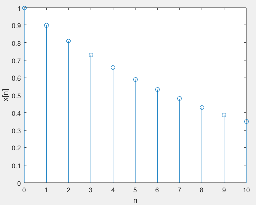
En el intervalo n1< no < n2. Por ejemplo, para implementar:

Usaremos la siguiente función de Matlab:

n=[0:10];;
x=(0.9).^n;
stem(n,x);
xlabel(‘n’); ylabel(‘x[n]’)

Este script genera:

Serie Geométrica

Una secuencia exponencial de un solo lado, de la forma:

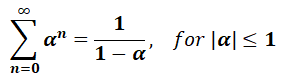
Donde α es una constante arbitraria. Esta secuencia es llamada a geometric series.  En PDS, la convergencia y la expresión para la suma de los componentes de esta serie are es utilizado en muchas aplicaciones. La serie converge para:

Mientras se cumpla esta condición, la suma de los componentes de la serie geométrica converge a:

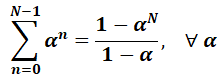
A partir de aquí, necesitamos además una expresión para la suma de cualquier número finito de términos de la serie, y está dado por:

Estos dos importantes resultados se utilizarán ampliamente en PDS.

Complex-valued exponential sequence

Where σ produces an attenuation (if<0) or amplification (if>0)  and ωo is the frequency in radians. The Matlab function exp generates the exponential sequences. For example, for x[n] =exp[(2+j3)n], 0n10, we will use the following script:

n=[0:10]; x=exp(3j*n);
stem(n,k)

This script yields:

Fuente:

  • Digital Signal Processing Using Matlab, 3erd ed

ANTERIOR:

También te puede interesar:

Revisión literaria hecha por:

Prof. Larry Francis Obando – Technical Specialist – Educational Content Writer

Se hacen trabajos, se resuelven ejercicios!!

WhatsApp:  +34633129287  Atención Inmediata!!

Twitter: @dademuch

Copywriting, Content Marketing, Tesis, Monografías, Paper Académicos, White Papers (Español – Inglés)

Escuela de Ingeniería Electrónica de la Universidad Simón Bolívar, USB Valle de Sartenejas.

Escuela de Ingeniería Eléctrica de la Universidad Central de Venezuela, UCV CCs

Escuela de Turismo de la Universidad Simón Bolívar, Núcleo Litoral.

Contacto: España. +34633129287

Caracas, Quito, Guayaquil, Jaén. 

WhatsApp:  +34633129287     

Twitter: @dademuch

FACEBOOK: DademuchConnection

email: dademuchconnection@gmail.com